how to write a multiple regression hypothesis

Save 10% on All AnalystPrep 2024 Study Packages with Coupon Code BLOG10 .

• Payment Plans
• Product List
• Partnerships

• Try Free Trial
• Study Packages
• Levels I, II & III Lifetime Package
• Video Lessons
• Study Notes
• Practice Questions
• Levels II & III Lifetime Package
• About the Exam
• About your Instructor
• Part I Study Packages
• Parts I & II Packages
• Part I & Part II Lifetime Package
• Part II Study Packages
• Exams P & FM Lifetime Package
• Quantitative Questions
• Verbal Questions
• Data Insight Questions
• Live Tutoring
• About your Instructors
• EA Practice Questions
• Data Sufficiency Questions
• Integrated Reasoning Questions

Hypothesis Tests and Confidence Intervals in Multiple Regression

After completing this reading you should be able to:

• Construct, apply, and interpret hypothesis tests and confidence intervals for a single coefficient in a multiple regression.
• Construct, apply, and interpret joint hypothesis tests and confidence intervals for multiple coefficients in a multiple regression.
• Interpret the \(F\)-statistic.
• Interpret tests of a single restriction involving multiple coefficients.
• Interpret confidence sets for multiple coefficients.
• Identify examples of omitted variable bias in multiple regressions.
• Interpret the \({ R }^{ 2 }\) and adjusted \({ R }^{ 2 }\) in a multiple regression.

Hypothesis Tests and Confidence Intervals for a Single Coefficient

This section is about the calculation of the standard error, hypotheses testing, and confidence interval construction for a single regression in a multiple regression equation.

Introduction

In a previous chapter, we looked at simple linear regression where we deal with just one regressor (independent variable). The response (dependent variable) is assumed to be affected by just one independent variable.  M ultiple regression, on the other hand ,  simultaneously considers the influence of multiple explanatory variables on a response variable Y. We may want to establish the confidence interval of one of the independent variables. We may want to evaluate whether any particular independent variable has a significant effect on the dependent variable. Finally, We may also want to establish whether the independent variables as a group have a significant effect on the dependent variable. In this chapter, we delve into ways all this can be achieved.

Hypothesis Tests for a single coefficient

Suppose that we are testing the hypothesis that the true coefficient \({ \beta }_{ j }\) on the \(j\)th regressor takes on some specific value \({ \beta }_{ j,0 }\). Let the alternative hypothesis be two-sided. Therefore, the following is the mathematical expression of the two hypotheses:

$$ { H }_{ 0 }:{ \beta }_{ j }={ \beta }_{ j,0 }\quad vs.\quad { H }_{ 1 }:{ \beta }_{ j }\neq { \beta }_{ j,0 } $$

This expression represents the two-sided alternative. The following are the steps to follow while testing the null hypothesis:

• Computing the coefficient’s standard error.

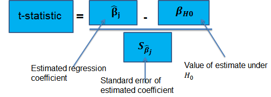
$$ p-value=2\Phi \left( -|{ t }^{ act }| \right) $$

• Also, the \(t\)-statistic can be compared to the critical value corresponding to the significance level that is desired for the test.

Confidence Intervals for a Single Coefficient

The confidence interval for a regression coefficient in multiple regression is calculated and interpreted the same way as it is in simple linear regression. 

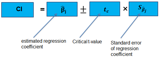
The t-statistic has n – k – 1 degrees of freedom where k = number of independents

Supposing that an interval contains the true value of \({ \beta }_{ j }\) with a probability of 95%. This is simply the 95% two-sided confidence interval for \({ \beta }_{ j }\). The implication here is that the true value of \({ \beta }_{ j }\) is contained in 95% of all possible randomly drawn variables.

Alternatively, the 95% two-sided confidence interval for \({ \beta }_{ j }\) is the set of values that are impossible to reject when a two-sided hypothesis test of 5% is applied. Therefore, with a large sample size:

$$ 95\%\quad confidence\quad interval\quad for\quad { \beta }_{ j }=\left[ { \hat { \beta } }_{ j }-1.96SE\left( { \hat { \beta } }_{ j } \right) ,{ \hat { \beta } }_{ j }+1.96SE\left( { \hat { \beta } }_{ j } \right) \right] $$

Tests of Joint Hypotheses

In this section, we consider the formulation of the joint hypotheses on multiple regression coefficients. We will further study the application of an \(F\)-statistic in their testing.

Hypotheses Testing on Two or More Coefficients

Joint null hypothesis.

In multiple regression, we canno t test the null hypothesis that all slope coefficients are equal 0 based on t -tests that each individual slope coefficient equals 0. Why? individual t-tests do not account for the effects of interactions among the independent variables.

For this reason, we conduct the F-test which uses the F-statistic .  The F-test tests the null hypothesis that all of the slope coefficients in the multiple regression model are jointly equal to 0, .i.e.,

\(F\)-Statistic

The F-statistic, which is always a one-tailed test , is calculated as:

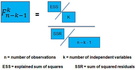
To determine whether at least one of the coefficients is statistically significant, the calculated F-statistic is compared with the one-tailed critical F-value, at the appropriate level of significance.

Decision rule:

Rejection of the null hypothesis at a stated level of significance indicates that at least one of the coefficients is significantly different than zero, i.e, at least one of the independent variables in the regression model makes a significant contribution to the dependent variable.

An analyst runs a regression of monthly value-stock returns on four independent variables over 48 months.

The total sum of squares for the regression is 360, and the sum of squared errors is 120.

Test the null hypothesis at the 5% significance level (95% confidence) that all the four independent variables are equal to zero.

\({ H }_{ 0 }:{ \beta }_{ 1 }=0,{ \beta }_{ 2 }=0,\dots ,{ \beta }_{ 4 }=0 \)

\({ H }_{ 1 }:{ \beta }_{ j }\neq 0\) (at least one j is not equal to zero, j=1,2… k )

ESS = TSS – SSR = 360 – 120 = 240

The calculated test statistic = (ESS/k)/(SSR/(n-k-1))

=(240/4)/(120/43) = 21.5

\({ F }_{ 43 }^{ 4 }\) is approximately 2.44 at 5% significance level.

Decision: Reject H 0 .

Conclusion: at least one of the 4 independents is significantly different than zero.

Omitted Variable Bias in Multiple Regression

This is the bias in the OLS estimator arising when at least one included regressor gets collaborated with an omitted variable. The following conditions must be satisfied for an omitted variable bias to occur:

• There must be a correlation between at least one of the included regressors and the omitted variable.
• The dependent variable \(Y\) must be determined by the omitted variable.

Practical Interpretation of the \({ R }^{ 2 }\) and the adjusted \({ R }^{ 2 }\), \({ \bar { R } }^{ 2 }\)

To determine the accuracy within which the OLS regression line fits the data, we apply the coefficient of determination and the regression’s standard error . 

The coefficient of determination, represented by \({ R }^{ 2 }\), is a measure of the “goodness of fit” of the regression. It is interpreted as the percentage of variation in the dependent variable explained by the independent variables

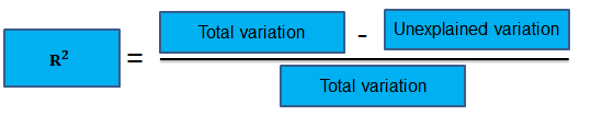
\({ R }^{ 2 }\) is not a reliable indicator of the explanatory power of a multiple regression model.Why? \({ R }^{ 2 }\) almost always increases as new independent variables are added to the model, even if the marginal contribution of the new variable is not statistically significant. Thus, a high \({ R }^{ 2 }\) may reflect the impact of a large set of independents rather than how well the set explains the dependent.This problem is solved by the use of the adjusted \({ R }^{ 2 }\) (extensively covered in chapter 8)

The following are the factors to watch out when guarding against applying the \({ R }^{ 2 }\) or the \({ \bar { R } }^{ 2 }\):

• An added variable doesn’t have to be statistically significant just because the \({ R }^{ 2 }\) or the \({ \bar { R } }^{ 2 }\) has increased.
• It is not always true that the regressors are a true cause of the dependent variable, just because there is a high \({ R }^{ 2 }\) or \({ \bar { R } }^{ 2 }\).
• It is not necessary that there is no omitted variable bias just because we have a high \({ R }^{ 2 }\) or \({ \bar { R } }^{ 2 }\).
• It is not necessarily true that we have the most appropriate set of regressors just because we have a high \({ R }^{ 2 }\) or \({ \bar { R } }^{ 2 }\).
• It is not necessarily true that we have an inappropriate set of regressors just because we have a low \({ R }^{ 2 }\) or \({ \bar { R } }^{ 2 }\).

An economist tests the hypothesis that GDP growth in a certain country can be explained by interest rates and inflation.

Using some 30 observations, the analyst formulates the following regression equation:

$$ GDP growth = { \hat { \beta } }_{ 0 } + { \hat { \beta } }_{ 1 } Interest+ { \hat { \beta } }_{ 2 } Inflation $$

Regression estimates are as follows:

Is the coefficient for interest rates significant at 5%?

• Since the test statistic < t-critical, we accept H 0 ; the interest rate coefficient is  not   significant at the 5% level.
• Since the test statistic > t-critical, we reject H 0 ; the interest rate coefficient is not significant at the 5% level.
• Since the test statistic > t-critical, we reject H 0 ; the interest rate coefficient is significant at the 5% level.
• Since the test statistic < t-critical, we accept H 1 ; the interest rate coefficient is significant at the 5% level.

The correct answer is  C .

We have GDP growth = 0.10 + 0.20(Int) + 0.15(Inf)

Hypothesis:

$$ { H }_{ 0 }:{ \hat { \beta } }_{ 1 } = 0 \quad vs \quad { H }_{ 1 }:{ \hat { \beta } }_{ 1 }≠0 $$

The test statistic is:

$$ t = \left( \frac { 0.20 – 0 }{ 0.05 } \right)  = 4 $$

The critical value is t (α/2, n-k-1) = t 0.025,27  = 2.052 (which can be found on the t-table).

Conclusion : The interest rate coefficient is significant at the 5% level.

Offered by AnalystPrep

Modeling Cycles: MA, AR, and ARMA Models

Empirical approaches to risk metrics and hedging, measuring return, volatility, and corr ....

After completing this reading, you should be able to: Calculate, distinguish, and convert... Read More

Machine Learning and Prediction

After completing this reading, you should be able to: Explain the role of... Read More

Binomial Trees

After completing this reading you should be able to: Calculate the value of... Read More

Applying the CAPM to Performance Measu ...

After completing this reading, you should be able to: Calculate, compare, and evaluate... Read More

Leave a Comment Cancel reply

You must be logged in to post a comment.

Multiple Regression Analysis using SPSS Statistics

Introduction.

Multiple regression is an extension of simple linear regression. It is used when we want to predict the value of a variable based on the value of two or more other variables. The variable we want to predict is called the dependent variable (or sometimes, the outcome, target or criterion variable). The variables we are using to predict the value of the dependent variable are called the independent variables (or sometimes, the predictor, explanatory or regressor variables).

For example, you could use multiple regression to understand whether exam performance can be predicted based on revision time, test anxiety, lecture attendance and gender. Alternately, you could use multiple regression to understand whether daily cigarette consumption can be predicted based on smoking duration, age when started smoking, smoker type, income and gender.

Multiple regression also allows you to determine the overall fit (variance explained) of the model and the relative contribution of each of the predictors to the total variance explained. For example, you might want to know how much of the variation in exam performance can be explained by revision time, test anxiety, lecture attendance and gender "as a whole", but also the "relative contribution" of each independent variable in explaining the variance.

This "quick start" guide shows you how to carry out multiple regression using SPSS Statistics, as well as interpret and report the results from this test. However, before we introduce you to this procedure, you need to understand the different assumptions that your data must meet in order for multiple regression to give you a valid result. We discuss these assumptions next.

SPSS Statistics

Assumptions.

When you choose to analyse your data using multiple regression, part of the process involves checking to make sure that the data you want to analyse can actually be analysed using multiple regression. You need to do this because it is only appropriate to use multiple regression if your data "passes" eight assumptions that are required for multiple regression to give you a valid result. In practice, checking for these eight assumptions just adds a little bit more time to your analysis, requiring you to click a few more buttons in SPSS Statistics when performing your analysis, as well as think a little bit more about your data, but it is not a difficult task.

Before we introduce you to these eight assumptions, do not be surprised if, when analysing your own data using SPSS Statistics, one or more of these assumptions is violated (i.e., not met). This is not uncommon when working with real-world data rather than textbook examples, which often only show you how to carry out multiple regression when everything goes well! However, don’t worry. Even when your data fails certain assumptions, there is often a solution to overcome this. First, let's take a look at these eight assumptions:

• Assumption #1: Your dependent variable should be measured on a continuous scale (i.e., it is either an interval or ratio variable). Examples of variables that meet this criterion include revision time (measured in hours), intelligence (measured using IQ score), exam performance (measured from 0 to 100), weight (measured in kg), and so forth. You can learn more about interval and ratio variables in our article: Types of Variable . If your dependent variable was measured on an ordinal scale, you will need to carry out ordinal regression rather than multiple regression. Examples of ordinal variables include Likert items (e.g., a 7-point scale from "strongly agree" through to "strongly disagree"), amongst other ways of ranking categories (e.g., a 3-point scale explaining how much a customer liked a product, ranging from "Not very much" to "Yes, a lot").
• Assumption #2: You have two or more independent variables , which can be either continuous (i.e., an interval or ratio variable) or categorical (i.e., an ordinal or nominal variable). For examples of continuous and ordinal variables , see the bullet above. Examples of nominal variables include gender (e.g., 2 groups: male and female), ethnicity (e.g., 3 groups: Caucasian, African American and Hispanic), physical activity level (e.g., 4 groups: sedentary, low, moderate and high), profession (e.g., 5 groups: surgeon, doctor, nurse, dentist, therapist), and so forth. Again, you can learn more about variables in our article: Types of Variable . If one of your independent variables is dichotomous and considered a moderating variable, you might need to run a Dichotomous moderator analysis .
• Assumption #3: You should have independence of observations (i.e., independence of residuals ), which you can easily check using the Durbin-Watson statistic, which is a simple test to run using SPSS Statistics. We explain how to interpret the result of the Durbin-Watson statistic, as well as showing you the SPSS Statistics procedure required, in our enhanced multiple regression guide.
• Assumption #4: There needs to be a linear relationship between (a) the dependent variable and each of your independent variables, and (b) the dependent variable and the independent variables collectively . Whilst there are a number of ways to check for these linear relationships, we suggest creating scatterplots and partial regression plots using SPSS Statistics, and then visually inspecting these scatterplots and partial regression plots to check for linearity. If the relationship displayed in your scatterplots and partial regression plots are not linear, you will have to either run a non-linear regression analysis or "transform" your data, which you can do using SPSS Statistics. In our enhanced multiple regression guide, we show you how to: (a) create scatterplots and partial regression plots to check for linearity when carrying out multiple regression using SPSS Statistics; (b) interpret different scatterplot and partial regression plot results; and (c) transform your data using SPSS Statistics if you do not have linear relationships between your variables.
• Assumption #5: Your data needs to show homoscedasticity , which is where the variances along the line of best fit remain similar as you move along the line. We explain more about what this means and how to assess the homoscedasticity of your data in our enhanced multiple regression guide. When you analyse your own data, you will need to plot the studentized residuals against the unstandardized predicted values. In our enhanced multiple regression guide, we explain: (a) how to test for homoscedasticity using SPSS Statistics; (b) some of the things you will need to consider when interpreting your data; and (c) possible ways to continue with your analysis if your data fails to meet this assumption.
• Assumption #6: Your data must not show multicollinearity , which occurs when you have two or more independent variables that are highly correlated with each other. This leads to problems with understanding which independent variable contributes to the variance explained in the dependent variable, as well as technical issues in calculating a multiple regression model. Therefore, in our enhanced multiple regression guide, we show you: (a) how to use SPSS Statistics to detect for multicollinearity through an inspection of correlation coefficients and Tolerance/VIF values; and (b) how to interpret these correlation coefficients and Tolerance/VIF values so that you can determine whether your data meets or violates this assumption.
• Assumption #7: There should be no significant outliers , high leverage points or highly influential points . Outliers, leverage and influential points are different terms used to represent observations in your data set that are in some way unusual when you wish to perform a multiple regression analysis. These different classifications of unusual points reflect the different impact they have on the regression line. An observation can be classified as more than one type of unusual point. However, all these points can have a very negative effect on the regression equation that is used to predict the value of the dependent variable based on the independent variables. This can change the output that SPSS Statistics produces and reduce the predictive accuracy of your results as well as the statistical significance. Fortunately, when using SPSS Statistics to run multiple regression on your data, you can detect possible outliers, high leverage points and highly influential points. In our enhanced multiple regression guide, we: (a) show you how to detect outliers using "casewise diagnostics" and "studentized deleted residuals", which you can do using SPSS Statistics, and discuss some of the options you have in order to deal with outliers; (b) check for leverage points using SPSS Statistics and discuss what you should do if you have any; and (c) check for influential points in SPSS Statistics using a measure of influence known as Cook's Distance, before presenting some practical approaches in SPSS Statistics to deal with any influential points you might have.
• Assumption #8: Finally, you need to check that the residuals (errors) are approximately normally distributed (we explain these terms in our enhanced multiple regression guide). Two common methods to check this assumption include using: (a) a histogram (with a superimposed normal curve) and a Normal P-P Plot; or (b) a Normal Q-Q Plot of the studentized residuals. Again, in our enhanced multiple regression guide, we: (a) show you how to check this assumption using SPSS Statistics, whether you use a histogram (with superimposed normal curve) and Normal P-P Plot, or Normal Q-Q Plot; (b) explain how to interpret these diagrams; and (c) provide a possible solution if your data fails to meet this assumption.

You can check assumptions #3, #4, #5, #6, #7 and #8 using SPSS Statistics. Assumptions #1 and #2 should be checked first, before moving onto assumptions #3, #4, #5, #6, #7 and #8. Just remember that if you do not run the statistical tests on these assumptions correctly, the results you get when running multiple regression might not be valid. This is why we dedicate a number of sections of our enhanced multiple regression guide to help you get this right. You can find out about our enhanced content as a whole on our Features: Overview page, or more specifically, learn how we help with testing assumptions on our Features: Assumptions page.

In the section, Procedure , we illustrate the SPSS Statistics procedure to perform a multiple regression assuming that no assumptions have been violated. First, we introduce the example that is used in this guide.

A health researcher wants to be able to predict "VO 2 max", an indicator of fitness and health. Normally, to perform this procedure requires expensive laboratory equipment and necessitates that an individual exercise to their maximum (i.e., until they can longer continue exercising due to physical exhaustion). This can put off those individuals who are not very active/fit and those individuals who might be at higher risk of ill health (e.g., older unfit subjects). For these reasons, it has been desirable to find a way of predicting an individual's VO 2 max based on attributes that can be measured more easily and cheaply. To this end, a researcher recruited 100 participants to perform a maximum VO 2 max test, but also recorded their "age", "weight", "heart rate" and "gender". Heart rate is the average of the last 5 minutes of a 20 minute, much easier, lower workload cycling test. The researcher's goal is to be able to predict VO 2 max based on these four attributes: age, weight, heart rate and gender.

Setup in SPSS Statistics

In SPSS Statistics, we created six variables: (1) VO 2 max , which is the maximal aerobic capacity; (2) age , which is the participant's age; (3) weight , which is the participant's weight (technically, it is their 'mass'); (4) heart_rate , which is the participant's heart rate; (5) gender , which is the participant's gender; and (6) caseno , which is the case number. The caseno variable is used to make it easy for you to eliminate cases (e.g., "significant outliers", "high leverage points" and "highly influential points") that you have identified when checking for assumptions. In our enhanced multiple regression guide, we show you how to correctly enter data in SPSS Statistics to run a multiple regression when you are also checking for assumptions. You can learn about our enhanced data setup content on our Features: Data Setup page. Alternately, see our generic, "quick start" guide: Entering Data in SPSS Statistics .

Test Procedure in SPSS Statistics

The seven steps below show you how to analyse your data using multiple regression in SPSS Statistics when none of the eight assumptions in the previous section, Assumptions , have been violated. At the end of these seven steps, we show you how to interpret the results from your multiple regression. If you are looking for help to make sure your data meets assumptions #3, #4, #5, #6, #7 and #8, which are required when using multiple regression and can be tested using SPSS Statistics, you can learn more in our enhanced guide (see our Features: Overview page to learn more).

Note: The procedure that follows is identical for SPSS Statistics versions 18 to 28 , as well as the subscription version of SPSS Statistics, with version 28 and the subscription version being the latest versions of SPSS Statistics. However, in version 27 and the subscription version , SPSS Statistics introduced a new look to their interface called " SPSS Light ", replacing the previous look for versions 26 and earlier versions , which was called " SPSS Standard ". Therefore, if you have SPSS Statistics versions 27 or 28 (or the subscription version of SPSS Statistics), the images that follow will be light grey rather than blue. However, the procedure is identical .

Published with written permission from SPSS Statistics, IBM Corporation.

Note: Don't worry that you're selecting A nalyze > R egression > L inear... on the main menu or that the dialogue boxes in the steps that follow have the title, Linear Regression . You have not made a mistake. You are in the correct place to carry out the multiple regression procedure. This is just the title that SPSS Statistics gives, even when running a multiple regression procedure.

Interpreting and Reporting the Output of Multiple Regression Analysis

SPSS Statistics will generate quite a few tables of output for a multiple regression analysis. In this section, we show you only the three main tables required to understand your results from the multiple regression procedure, assuming that no assumptions have been violated. A complete explanation of the output you have to interpret when checking your data for the eight assumptions required to carry out multiple regression is provided in our enhanced guide. This includes relevant scatterplots and partial regression plots, histogram (with superimposed normal curve), Normal P-P Plot and Normal Q-Q Plot, correlation coefficients and Tolerance/VIF values, casewise diagnostics and studentized deleted residuals.

However, in this "quick start" guide, we focus only on the three main tables you need to understand your multiple regression results, assuming that your data has already met the eight assumptions required for multiple regression to give you a valid result:

Determining how well the model fits

The first table of interest is the Model Summary table. This table provides the R , R 2 , adjusted R 2 , and the standard error of the estimate, which can be used to determine how well a regression model fits the data:

The " R " column represents the value of R , the multiple correlation coefficient . R can be considered to be one measure of the quality of the prediction of the dependent variable; in this case, VO 2 max . A value of 0.760, in this example, indicates a good level of prediction. The " R Square " column represents the R 2 value (also called the coefficient of determination), which is the proportion of variance in the dependent variable that can be explained by the independent variables (technically, it is the proportion of variation accounted for by the regression model above and beyond the mean model). You can see from our value of 0.577 that our independent variables explain 57.7% of the variability of our dependent variable, VO 2 max . However, you also need to be able to interpret " Adjusted R Square " ( adj. R 2 ) to accurately report your data. We explain the reasons for this, as well as the output, in our enhanced multiple regression guide.

Statistical significance

The F -ratio in the ANOVA table (see below) tests whether the overall regression model is a good fit for the data. The table shows that the independent variables statistically significantly predict the dependent variable, F (4, 95) = 32.393, p < .0005 (i.e., the regression model is a good fit of the data).

Estimated model coefficients

The general form of the equation to predict VO 2 max from age , weight , heart_rate , gender , is:

predicted VO 2 max = 87.83 – (0.165 x age ) – (0.385 x weight ) – (0.118 x heart_rate ) + (13.208 x gender )

This is obtained from the Coefficients table, as shown below:

Unstandardized coefficients indicate how much the dependent variable varies with an independent variable when all other independent variables are held constant. Consider the effect of age in this example. The unstandardized coefficient, B 1 , for age is equal to -0.165 (see Coefficients table). This means that for each one year increase in age, there is a decrease in VO 2 max of 0.165 ml/min/kg.

Statistical significance of the independent variables

You can test for the statistical significance of each of the independent variables. This tests whether the unstandardized (or standardized) coefficients are equal to 0 (zero) in the population. If p < .05, you can conclude that the coefficients are statistically significantly different to 0 (zero). The t -value and corresponding p -value are located in the " t " and " Sig. " columns, respectively, as highlighted below:

You can see from the " Sig. " column that all independent variable coefficients are statistically significantly different from 0 (zero). Although the intercept, B 0 , is tested for statistical significance, this is rarely an important or interesting finding.

Putting it all together

You could write up the results as follows:

A multiple regression was run to predict VO 2 max from gender, age, weight and heart rate. These variables statistically significantly predicted VO 2 max, F (4, 95) = 32.393, p < .0005, R 2 = .577. All four variables added statistically significantly to the prediction, p < .05.

If you are unsure how to interpret regression equations or how to use them to make predictions, we discuss this in our enhanced multiple regression guide. We also show you how to write up the results from your assumptions tests and multiple regression output if you need to report this in a dissertation/thesis, assignment or research report. We do this using the Harvard and APA styles. You can learn more about our enhanced content on our Features: Overview page.

Statistics Resources

• Excel - Tutorials
• Basic Probability Rules
• Single Event Probability
• Complement Rule
• Intersections & Unions
• Compound Events
• Levels of Measurement
• Independent and Dependent Variables
• Entering Data
• Central Tendency
• Data and Tests
• Displaying Data
• Discussing Statistics In-text
• SEM and Confidence Intervals
• Two-Way Frequency Tables
• Empirical Rule
• Finding Probability
• Accessing SPSS
• Chart and Graphs
• Frequency Table and Distribution
• Descriptive Statistics
• Converting Raw Scores to Z-Scores
• Converting Z-scores to t-scores
• Split File/Split Output
• Partial Eta Squared
• Downloading and Installing G*Power: Windows/PC
• Correlation
• Testing Parametric Assumptions
• One-Way ANOVA
• Two-Way ANOVA
• Repeated Measures ANOVA
• Goodness-of-Fit
• Test of Association
• Pearson's r
• Point Biserial
• Mediation and Moderation
• Simple Linear Regression

Multiple Linear Regression

• Binomial Logistic Regression
• Multinomial Logistic Regression
• Independent Samples T-test
• Dependent Samples T-test
• Testing Assumptions
• T-tests using SPSS
• T-Test Practice
• Predictive Analytics This link opens in a new window
• Quantitative Research Questions
• Null & Alternative Hypotheses
• One-Tail vs. Two-Tail
• Alpha & Beta
• Associated Probability
• Decision Rule
• Statement of Conclusion
• Statistics Group Sessions

The multiple regression analysis expands the simple linear regression to allow for multiple independent (predictor) variables. The model created now includes two or more predictor variables, but still contains a single dependent (criterion) variable.

Assumptions

• Dependent variable is continuous (interval or ratio)
• Independent variables are continuous (interval or ratio) or categorical (nominal or ordinal)
• Independence of observations - assessed using Durbin-Waston statistic
• Linear relationship between the dependent variable and  each  independent variable - visual exam of scatterplots
• Homoscedasticity - assessed through a visual examination of a scatterplot of the residuals
• No multicollinearity (high correlation between independent variables) - inspection of correlation values and tolerance values
• No outliers or highly influential points - outliers can be detected using casewise diagnostics and studentized deleted residuals
• Residuals are approximately normally distributed - checked using histogram, P-P Plot, or Q-Q Plot of residuals.

Running Multiple Linear Regression in SPSS

• Analyze > Regression > Linear...
• Place all independent variables in the "Independent(s)" box and the dependent variable in the "Dependent" box
• Click on the "Statistics" button to select options for testing assumptions. Click "Continue" to go back to main box.
• Click "OK" to generate the results.

Interpreting Output

• R = multiple correlation coefficient
• R-Square = coefficient of determination - measure of variance accounted for by the model
• Adjusted R-Square = measure of variance accounted for by the model adjusted for the number of independent variables in the model
• F-ratio = measure of how effective the independent variables, collectively, are at predicting the dependent variable
• Sig. (associated probability) = provides the probability of obtaining the F-ratio by chance
• Unstandardized B(eta) = measure of how much the dependent variable varies with changes in one independent variable is changed when all other variables are held constant = used to create the multiple regression equation for predicting the outcome variable.
• t and Sig. = used to determine the significance of each independent variable in the model

Reporting Results in APA Style

A multiple regression was run to predict job satisfaction from salary, years of experience, and perceived appreciation. This resulted in a significant model,  F (3, 72) = 16.2132,  p  < .01,  R2  = .638. The individual predictors were examined further and indicated that salary ( t  = 9.21, p  < .01) and perceived appreciation ( t  = 15.329,  p  < .001) were significant predictors but, years of experience was not ( t  = 1.16,  p  = .135).

Was this resource helpful?

• << Previous: Simple Linear Regression
• Next: Binomial Logistic Regression >>
• Last Updated: Apr 19, 2024 3:09 PM
• URL: https://resources.nu.edu/statsresources

• school Campus Bookshelves
• menu_book Bookshelves
• perm_media Learning Objects
• login Login
• how_to_reg Request Instructor Account
• hub Instructor Commons

Margin Size

• Download Page (PDF)
• Download Full Book (PDF)
• Periodic Table
• Physics Constants
• Scientific Calculator
• Reference & Cite
• Tools expand_more
• Readability

selected template will load here

This action is not available.

12.2.1: Hypothesis Test for Linear Regression

• Last updated
• Save as PDF
• Page ID 34850

• Rachel Webb
• Portland State University

\( \newcommand{\vecs}[1]{\overset { \scriptstyle \rightharpoonup} {\mathbf{#1}} } \)

\( \newcommand{\vecd}[1]{\overset{-\!-\!\rightharpoonup}{\vphantom{a}\smash {#1}}} \)

\( \newcommand{\id}{\mathrm{id}}\) \( \newcommand{\Span}{\mathrm{span}}\)

( \newcommand{\kernel}{\mathrm{null}\,}\) \( \newcommand{\range}{\mathrm{range}\,}\)

\( \newcommand{\RealPart}{\mathrm{Re}}\) \( \newcommand{\ImaginaryPart}{\mathrm{Im}}\)

\( \newcommand{\Argument}{\mathrm{Arg}}\) \( \newcommand{\norm}[1]{\| #1 \|}\)

\( \newcommand{\inner}[2]{\langle #1, #2 \rangle}\)

\( \newcommand{\Span}{\mathrm{span}}\)

\( \newcommand{\id}{\mathrm{id}}\)

\( \newcommand{\kernel}{\mathrm{null}\,}\)

\( \newcommand{\range}{\mathrm{range}\,}\)

\( \newcommand{\RealPart}{\mathrm{Re}}\)

\( \newcommand{\ImaginaryPart}{\mathrm{Im}}\)

\( \newcommand{\Argument}{\mathrm{Arg}}\)

\( \newcommand{\norm}[1]{\| #1 \|}\)

\( \newcommand{\Span}{\mathrm{span}}\) \( \newcommand{\AA}{\unicode[.8,0]{x212B}}\)

\( \newcommand{\vectorA}[1]{\vec{#1}}      % arrow\)

\( \newcommand{\vectorAt}[1]{\vec{\text{#1}}}      % arrow\)

\( \newcommand{\vectorB}[1]{\overset { \scriptstyle \rightharpoonup} {\mathbf{#1}} } \)

\( \newcommand{\vectorC}[1]{\textbf{#1}} \)

\( \newcommand{\vectorD}[1]{\overrightarrow{#1}} \)

\( \newcommand{\vectorDt}[1]{\overrightarrow{\text{#1}}} \)

\( \newcommand{\vectE}[1]{\overset{-\!-\!\rightharpoonup}{\vphantom{a}\smash{\mathbf {#1}}}} \)

To test to see if the slope is significant we will be doing a two-tailed test with hypotheses. The population least squares regression line would be \(y = \beta_{0} + \beta_{1} + \varepsilon\) where \(\beta_{0}\) (pronounced “beta-naught”) is the population \(y\)-intercept, \(\beta_{1}\) (pronounced “beta-one”) is the population slope and \(\varepsilon\) is called the error term.

If the slope were horizontal (equal to zero), the regression line would give the same \(y\)-value for every input of \(x\) and would be of no use. If there is a statistically significant linear relationship then the slope needs to be different from zero. We will only do the two-tailed test, but the same rules for hypothesis testing apply for a one-tailed test.

We will only be using the two-tailed test for a population slope.

The hypotheses are:

\(H_{0}: \beta_{1} = 0\) \(H_{1}: \beta_{1} \neq 0\)

The null hypothesis of a two-tailed test states that there is not a linear relationship between \(x\) and \(y\). The alternative hypothesis of a two-tailed test states that there is a significant linear relationship between \(x\) and \(y\).

Either a t-test or an F-test may be used to see if the slope is significantly different from zero. The population of the variable \(y\) must be normally distributed.

F-Test for Regression

An F-test can be used instead of a t-test. Both tests will yield the same results, so it is a matter of preference and what technology is available. Figure 12-12 is a template for a regression ANOVA table,

where \(n\) is the number of pairs in the sample and \(p\) is the number of predictor (independent) variables; for now this is just \(p = 1\). Use the F-distribution with degrees of freedom for regression = \(df_{R} = p\), and degrees of freedom for error = \(df_{E} = n - p - 1\). This F-test is always a right-tailed test since ANOVA is testing the variation in the regression model is larger than the variation in the error.

Use an F-test to see if there is a significant relationship between hours studied and grade on the exam. Use \(\alpha\) = 0.05.

T-Test for Regression

If the regression equation has a slope of zero, then every \(x\) value will give the same \(y\) value and the regression equation would be useless for prediction. We should perform a t-test to see if the slope is significantly different from zero before using the regression equation for prediction. The numeric value of t will be the same as the t-test for a correlation. The two test statistic formulas are algebraically equal; however, the formulas are different and we use a different parameter in the hypotheses.

The formula for the t-test statistic is \(t = \frac{b_{1}}{\sqrt{ \left(\frac{MSE}{SS_{xx}}\right) }}\)

Use the t-distribution with degrees of freedom equal to \(n - p - 1\).

The t-test for slope has the same hypotheses as the F-test:

Use a t-test to see if there is a significant relationship between hours studied and grade on the exam, use \(\alpha\) = 0.05.

Statistics Made Easy

Understanding the Null Hypothesis for Linear Regression

Linear regression is a technique we can use to understand the relationship between one or more predictor variables and a response variable .

If we only have one predictor variable and one response variable, we can use simple linear regression , which uses the following formula to estimate the relationship between the variables:

ŷ = β 0 + β 1 x

• ŷ: The estimated response value.
• β 0 : The average value of y when x is zero.
• β 1 : The average change in y associated with a one unit increase in x.
• x: The value of the predictor variable.

Simple linear regression uses the following null and alternative hypotheses:

• H 0 : β 1 = 0
• H A : β 1 ≠ 0

The null hypothesis states that the coefficient β 1 is equal to zero. In other words, there is no statistically significant relationship between the predictor variable, x, and the response variable, y.

The alternative hypothesis states that β 1 is not equal to zero. In other words, there is a statistically significant relationship between x and y.

If we have multiple predictor variables and one response variable, we can use multiple linear regression , which uses the following formula to estimate the relationship between the variables:

ŷ = β 0 + β 1 x 1 + β 2 x 2 + … + β k x k

• β 0 : The average value of y when all predictor variables are equal to zero.
• β i : The average change in y associated with a one unit increase in x i .
• x i : The value of the predictor variable x i .

Multiple linear regression uses the following null and alternative hypotheses:

• H 0 : β 1 = β 2 = … = β k = 0
• H A : β 1 = β 2 = … = β k ≠ 0

The null hypothesis states that all coefficients in the model are equal to zero. In other words, none of the predictor variables have a statistically significant relationship with the response variable, y.

The alternative hypothesis states that not every coefficient is simultaneously equal to zero.

The following examples show how to decide to reject or fail to reject the null hypothesis in both simple linear regression and multiple linear regression models.

Example 1: Simple Linear Regression

Suppose a professor would like to use the number of hours studied to predict the exam score that students will receive in his class. He collects data for 20 students and fits a simple linear regression model.

The following screenshot shows the output of the regression model:

The fitted simple linear regression model is:

Exam Score = 67.1617 + 5.2503*(hours studied)

To determine if there is a statistically significant relationship between hours studied and exam score, we need to analyze the overall F value of the model and the corresponding p-value:

• Overall F-Value:  47.9952
• P-value:  0.000

Since this p-value is less than .05, we can reject the null hypothesis. In other words, there is a statistically significant relationship between hours studied and exam score received.

Example 2: Multiple Linear Regression

Suppose a professor would like to use the number of hours studied and the number of prep exams taken to predict the exam score that students will receive in his class. He collects data for 20 students and fits a multiple linear regression model.

The fitted multiple linear regression model is:

Exam Score = 67.67 + 5.56*(hours studied) – 0.60*(prep exams taken)

To determine if there is a jointly statistically significant relationship between the two predictor variables and the response variable, we need to analyze the overall F value of the model and the corresponding p-value:

• Overall F-Value:  23.46
• P-value:  0.00

Since this p-value is less than .05, we can reject the null hypothesis. In other words, hours studied and prep exams taken have a jointly statistically significant relationship with exam score.

Note: Although the p-value for prep exams taken (p = 0.52) is not significant, prep exams combined with hours studied has a significant relationship with exam score.

Additional Resources

Understanding the F-Test of Overall Significance in Regression How to Read and Interpret a Regression Table How to Report Regression Results How to Perform Simple Linear Regression in Excel How to Perform Multiple Linear Regression in Excel

Featured Posts

Hey there. My name is Zach Bobbitt. I have a Masters of Science degree in Applied Statistics and I’ve worked on machine learning algorithms for professional businesses in both healthcare and retail. I’m passionate about statistics, machine learning, and data visualization and I created Statology to be a resource for both students and teachers alike.  My goal with this site is to help you learn statistics through using simple terms, plenty of real-world examples, and helpful illustrations.

2 Replies to “Understanding the Null Hypothesis for Linear Regression”

Thank you Zach, this helped me on homework!

Great articles, Zach.

I would like to cite your work in a research paper.

Could you provide me with your last name and initials.

Leave a Reply Cancel reply

Your email address will not be published. Required fields are marked *

Join the Statology Community

Sign up to receive Statology's exclusive study resource: 100 practice problems with step-by-step solutions. Plus, get our latest insights, tutorials, and data analysis tips straight to your inbox!

By subscribing you accept Statology's Privacy Policy.

Want to create or adapt books like this? Learn more about how Pressbooks supports open publishing practices.

Section 5.4: Hierarchical Regression Explanation, Assumptions, Interpretation, and Write Up

Learning Objectives

At the end of this section you should be able to answer the following questions:

• Explain how hierarchical regression differs from multiple regression.
• Discuss where you would use “control variables” in a hierarchical regression analyses.

Hierarchical Regression Explanation and Assumptions

Hierarchical regression is a type of regression model in which the predictors are entered in blocks. Each block represents one step (or model). The order (or which predictor goes into which block) to enter predictors into the model is decided by the researcher, but should always be based on theory.

The first block entered into a hierarchical regression can include “control variables,” which are variables that we want to hold constant. In a sense, researchers want to account for the variability of the control variables by removing it before analysing the relationship between the predictors and the outcome.

The example research question is “what is the effect of perceived stress on physical illness, after controlling for age and gender?”.  To answer this research question, we will need two blocks. One with age and gender, then the next block including perceived stress.

It is important to note that the assumptions for hierarchical regression are the same as those covered for simple or basic multiple regression. You may wish to go back to the section on multiple regression assumptions if you can’t remember the assumptions or want to check them out before progressing through the chapter.

Hierarchical Regression Interpretation

PowerPoint: Hierarchical Regression

For this example, please click on the link for Chapter Five – Hierarchical Regression below. You will find 4 slides that we will be referring to for the rest of this section.

• Chapter Five – Hierarchical Regression

For this test, the statistical program used was Jamovi, which is freely available to use. The first two slides show the steps to get produce the results. The third slide shows the output with any highlighting. You might want to think about what you have already learned, to see if you can work out the important elements of this output.

Slide 2 shows the overall model statistics. The first model, with only age and gender, can be seen circled in red. This model is obviously significant. The second model (circled in green) includes age, gender, and perceived stress. As you can see, the F statistic is larger for the second model. However, does this mean it is significantly larger?

To answer this question, we will need to look at the model change statistics on Slide 3. The R value for model 1 can be seen here circled in red as .202. This model explains approximately 4% of the variance in physical illness. The R value for model 2 is circled in green, and explains a more sizeable part of the variance, about 25%.

The significance of the change in the model can be seen in blue on Slide 3. The information you are looking at is the R squared change, the F statistic change, and the statistical significance of this change.

On Slide 4, you can examine the role of each individual independent variable on the dependant variable. For model one, as circled in red, age and gender are both significantly associated with physical illness. In this case, age is negatively associated (i.e. the younger you are, the more likely you are to be healthy), and gender is positively associated (in this case being female is more likely to result in more physical illness).  For model 2, gender is still positively associated and now perceived stress is also positively associated. However, age is no longer significantly associated with physical illness following the introduction of perceived stress. Possibly this is because older persons are experiencing less life stress than younger persons.

Hierarchical Regression Write Up

An example write up of a hierarchal regression analysis is seen below:

In order to test the predictions, a hierarchical multiple regression was conducted, with two blocks of variables. The first block included age and gender (0 = male, 1 = female) as the predictors, with difficulties in physical illness as the dependant variable. In block two, levels of perceived stress was also included as the predictor variable, with difficulties in perceived stress as the dependant variable.

Overall, the results showed that the first model was significant F (2,364) = 7.75, p = .001, R 2 =.04. Both age and gender were significantly associated with perceived life stress ( b =-0.14, t = -2.78, p = .006, and b =.14, t = 2.70, p = .007, respectively). The second model ( F (3,363) = 39.61, p < .001, R 2 =.25), which included physical illness ( b =0.47, t = 9.96, p < .001) showed significant improvement from the first model ∆ F (1,363) = 99.13, p < .001, ∆R 2 =.21,  , Overall, when age and location of participants were included in the model, the variables explained 8.6% of the variance, with the final model, including physical illness accounted for 24.7% of the variance, with model one and two representing a small, and large effect size, respectively.

Statistics for Research Students Copyright © 2022 by University of Southern Queensland is licensed under a Creative Commons Attribution 4.0 International License , except where otherwise noted.

Share This Book

Adverse pregnancy outcomes and coronary artery disease risk: A negative control Mendelian randomization study

• Find this author on Google Scholar
• Find this author on PubMed
• Search for this author on this site
• ORCID record for Tormod Rogne
• For correspondence: [email protected]
• ORCID record for Dipender Gill
• Info/History
• Supplementary material
• Preview PDF

Background Adverse pregnancy outcomes are predictive for future cardiovascular disease risk, but it is unclear whether they play a causal role. We conducted a Mendelian randomization study with males as a negative control population to estimate the associations between genetic liability to adverse pregnancy outcomes and risk of coronary artery disease.

Methods We extracted uncorrelated (R 2 <0.01) single-nucleotide polymorphisms strongly associated (p-value<5e-8) with miscarriage, gestational diabetes, hypertensive disorders of pregnancy, preeclampsia, placental abruption, poor fetal growth and preterm birth from relevant genome-wide association studies. Genetic associations with risk of coronary artery disease were extracted separately for females and males. The main analysis was the inverse-variance weighted analysis, while MR Egger, weighted median and weighted mode regression, bidirectional analyses, and the negative control population with males were sensitivity analyses to evaluate bias due to genetic pleiotropy.

Results The number of cases for the adverse pregnancy outcomes ranged from 691 (182,824 controls) for placental abruption to 49,996 (174,109 controls) for miscarriage, and there were 22,997 (310,499 controls) and 54,083 (240,453 controls) cases of coronary artery disease for females and males, respectively. We observed an association between genetic liability to hypertensive disorders of pregnancy and preeclampsia, and to some extent gestational diabetes, poor fetal growth and preterm birth, with an increased risk of coronary artery disease among females, which was supported by the MR Egger, weighted median and weighted mode regressions. However, in the negative control population of males, we observed largely the same associations as for females.

Conclusions The associations between adverse pregnancy outcomes and coronary artery disease risk were likely driven by confounding (e.g., shared genetic liability). Thus, our study does not support the hypothesis that adverse pregnancy outcomes are causal risk factors for cardiovascular diseases.

Competing Interest Statement

The authors have declared no competing interest.

Funding Statement

TR was funded by CTSA Grant Number UL1 TR001863 from the National Center for Advancing Translational Science (NCATS), a component of the National Institutes of Health (NIH). The contents of this manuscript are solely the responsibility of the authors and do not necessarily represent the official views of NIH. DG is supported by the British Heart Foundation Centre of Research Excellence at Imperial College London (RE/18/4/34215).

Author Declarations

I confirm all relevant ethical guidelines have been followed, and any necessary IRB and/or ethics committee approvals have been obtained.

I confirm that all necessary patient/participant consent has been obtained and the appropriate institutional forms have been archived, and that any patient/participant/sample identifiers included were not known to anyone (e.g., hospital staff, patients or participants themselves) outside the research group so cannot be used to identify individuals.

I understand that all clinical trials and any other prospective interventional studies must be registered with an ICMJE-approved registry, such as ClinicalTrials.gov. I confirm that any such study reported in the manuscript has been registered and the trial registration ID is provided (note: if posting a prospective study registered retrospectively, please provide a statement in the trial ID field explaining why the study was not registered in advance).

I have followed all appropriate research reporting guidelines, such as any relevant EQUATOR Network research reporting checklist(s) and other pertinent material, if applicable.

( dipender.gill{at}imperial.ac.uk )

Conflict of interest: All authors report no conflict of interest.

Funding/Support: TR was funded by CTSA Grant Number UL1 TR001863 from the National Center for Advancing Translational Science (NCATS), a component of the National Institutes of Health (NIH). The contents of this manuscript are solely the responsibility of the authors and do not necessarily represent the official views of NIH. DG is supported by the British Heart Foundation Centre of Research Excellence at Imperial College London (RE/18/4/34215).

Data Availability

All data used in the present study are publicly available.

View the discussion thread.

Supplementary Material

Thank you for your interest in spreading the word about medRxiv.

NOTE: Your email address is requested solely to identify you as the sender of this article.

Citation Manager Formats

• EndNote (tagged)
• EndNote 8 (xml)
• RefWorks Tagged
• Ref Manager
• Tweet Widget
• Facebook Like
• Google Plus One

Subject Area

• Cardiovascular Medicine
• Addiction Medicine (324)
• Allergy and Immunology (629)
• Anesthesia (166)
• Cardiovascular Medicine (2391)
• Dentistry and Oral Medicine (289)
• Dermatology (207)
• Emergency Medicine (380)
• Endocrinology (including Diabetes Mellitus and Metabolic Disease) (843)
• Epidemiology (11786)
• Forensic Medicine (10)
• Gastroenterology (703)
• Genetic and Genomic Medicine (3759)
• Geriatric Medicine (350)
• Health Economics (636)
• Health Informatics (2403)
• Health Policy (935)
• Health Systems and Quality Improvement (902)
• Hematology (341)
• HIV/AIDS (783)
• Infectious Diseases (except HIV/AIDS) (13330)
• Intensive Care and Critical Care Medicine (769)
• Medical Education (366)
• Medical Ethics (105)
• Nephrology (400)
• Neurology (3517)
• Nursing (199)
• Nutrition (528)
• Obstetrics and Gynecology (677)
• Occupational and Environmental Health (665)
• Oncology (1828)
• Ophthalmology (538)
• Orthopedics (219)
• Otolaryngology (287)
• Pain Medicine (234)
• Palliative Medicine (66)
• Pathology (447)
• Pediatrics (1035)
• Pharmacology and Therapeutics (426)
• Primary Care Research (423)
• Psychiatry and Clinical Psychology (3186)
• Public and Global Health (6161)
• Radiology and Imaging (1283)
• Rehabilitation Medicine and Physical Therapy (750)
• Respiratory Medicine (830)
• Rheumatology (379)
• Sexual and Reproductive Health (372)
• Sports Medicine (324)
• Surgery (402)
• Toxicology (50)
• Transplantation (172)
• Urology (146)