This browser is no longer supported.
Upgrade to Microsoft Edge to take advantage of the latest features, security updates, and technical support.

Machine learning tasks in ML.NET
- 14 contributors
A machine learning task is the type of prediction or inference being made, based on the problem or question that is being asked, and the available data. For example, the classification task assigns data to categories, and the clustering task groups data according to similarity.
Machine learning tasks rely on patterns in the data rather than being explicitly programmed.
This article describes the different machine learning tasks that you can choose from in ML.NET and some common use cases.
Once you have decided which task works for your scenario, then you need to choose the best algorithm to train your model. The available algorithms are listed in the section for each task.
Binary classification
A supervised machine learning task that is used to predict which of two classes (categories) an instance of data belongs to. The input of a classification algorithm is a set of labeled examples, where each label is an integer of either 0 or 1. The output of a binary classification algorithm is a classifier, which you can use to predict the class of new unlabeled instances. Examples of binary classification scenarios include:
- Understanding sentiment of Twitter comments as either "positive" or "negative".
- Diagnosing whether a patient has a certain disease or not.
- Making a decision to mark an email as "spam" or not.
- Determining if a photo contains a particular item or not, such as a dog or fruit.
For more information, see the Binary classification article on Wikipedia.
Binary classification trainers
You can train a binary classification model using the following algorithms:
- AveragedPerceptronTrainer
- SdcaLogisticRegressionBinaryTrainer
- SdcaNonCalibratedBinaryTrainer
- SymbolicSgdLogisticRegressionBinaryTrainer
- LbfgsLogisticRegressionBinaryTrainer
- LightGbmBinaryTrainer
- FastTreeBinaryTrainer
- FastForestBinaryTrainer
- GamBinaryTrainer
- FieldAwareFactorizationMachineTrainer
- PriorTrainer
- LinearSvmTrainer
Binary classification inputs and outputs
For best results with binary classification, the training data should be balanced (that is, equal numbers of positive and negative training data). Missing values should be handled before training.
The input label column data must be Boolean . The input features column data must be a fixed-size vector of Single .
These trainers output the following columns:
| Output Column Name | Column Type | Description |
|---|---|---|
| The raw score that was calculated by the model | ||
| The predicted label, based on the sign of the score. A negative score maps to and a positive score maps to . |
Multiclass classification
A supervised machine learning task that is used to predict the class (category) of an instance of data. The input of a classification algorithm is a set of labeled examples. Each label normally starts as text. It is then run through the TermTransform, which converts it to the Key (numeric) type. The output of a classification algorithm is a classifier, which you can use to predict the class of new unlabeled instances. Examples of multi-class classification scenarios include:
- Categorizing flights as "early", "on time", or "late".
- Understanding movie reviews as "positive", "neutral", or "negative".
- Categorizing hotel reviews as "location", "price", "cleanliness", etc.
For more information, see the Multiclass classification article on Wikipedia.
One vs all upgrades any binary classification learner to act on multiclass datasets. More information on Wikipedia .
Multiclass classification trainers
You can train a multiclass classification model using the following training algorithms:
- LightGbmMulticlassTrainer
- SdcaMaximumEntropyMulticlassTrainer
- SdcaNonCalibratedMulticlassTrainer
- LbfgsMaximumEntropyMulticlassTrainer
- NaiveBayesMulticlassTrainer
- OneVersusAllTrainer
- PairwiseCouplingTrainer
Multiclass classification inputs and outputs
The input label column data must be key type. The feature column must be a fixed size vector of Single .
This trainer outputs the following:
| Output Name | Type | Description |
|---|---|---|
| Vector of | The scores of all classes. Higher value means higher probability to fall into the associated class. If the i-th element has the largest value, the predicted label index would be i. Note that i is zero-based index. | |
| type | The predicted label's index. If its value is i, the actual label would be the i-th category in the key-valued input label type. |
A supervised machine learning task that is used to predict the value of the label from a set of related features. The label can be of any real value and is not from a finite set of values as in classification tasks. Regression algorithms model the dependency of the label on its related features to determine how the label will change as the values of the features are varied. The input of a regression algorithm is a set of examples with labels of known values. The output of a regression algorithm is a function, which you can use to predict the label value for any new set of input features. Examples of regression scenarios include:
- Predicting house prices based on house attributes such as number of bedrooms, location, or size.
- Predicting future stock prices based on historical data and current market trends.
- Predicting sales of a product based on advertising budgets.
Regression trainers
You can train a regression model using the following algorithms:
- LbfgsPoissonRegressionTrainer
- LightGbmRegressionTrainer
- SdcaRegressionTrainer
- OnlineGradientDescentTrainer
- FastTreeRegressionTrainer
- FastTreeTweedieTrainer
- FastForestRegressionTrainer
- GamRegressionTrainer
Regression inputs and outputs
The input label column data must be Single .
The trainers for this task output the following:
| Output Name | Type | Description |
|---|---|---|
| The raw score that was predicted by the model |
An unsupervised machine learning task that is used to group instances of data into clusters that contain similar characteristics. Clustering can also be used to identify relationships in a dataset that you might not logically derive by browsing or simple observation. The inputs and outputs of a clustering algorithm depends on the methodology chosen. You can take a distribution, centroid, connectivity, or density-based approach. ML.NET currently supports a centroid-based approach using K-Means clustering. Examples of clustering scenarios include:
- Understanding segments of hotel guests based on habits and characteristics of hotel choices.
- Identifying customer segments and demographics to help build targeted advertising campaigns.
- Categorizing inventory based on manufacturing metrics.
Clustering trainer
You can train a clustering model using the following algorithm:
- KMeansTrainer
Clustering inputs and outputs
The input features data must be Single . No labels are needed.
| Output Name | Type | Description |
|---|---|---|
| vector of | The distances of the given data point to all clusters' centroids | |
| type | The closest cluster's index predicted by the model. |
Anomaly detection
This task creates an anomaly detection model by using Principal Component Analysis (PCA). PCA-Based Anomaly Detection helps you build a model in scenarios where it is easy to obtain training data from one class, such as valid transactions, but difficult to obtain sufficient samples of the targeted anomalies.
An established technique in machine learning, PCA is frequently used in exploratory data analysis because it reveals the inner structure of the data and explains the variance in the data. PCA works by analyzing data that contains multiple variables. It looks for correlations among the variables and determines the combination of values that best captures differences in outcomes. These combined feature values are used to create a more compact feature space called the principal components.
Anomaly detection encompasses many important tasks in machine learning:
- Identifying transactions that are potentially fraudulent.
- Learning patterns that indicate that a network intrusion has occurred.
- Finding abnormal clusters of patients.
- Checking values entered into a system.
Because anomalies are rare events by definition, it can be difficult to collect a representative sample of data to use for modeling. The algorithms included in this category have been especially designed to address the core challenges of building and training models by using imbalanced data sets.
Anomaly detection trainer
You can train an anomaly detection model using the following algorithm:
- RandomizedPcaTrainer
Anomaly detection inputs and outputs
The input features must be a fixed-sized vector of Single .
| Output Name | Type | Description |
|---|---|---|
| The non-negative, unbounded score that was calculated by the anomaly detection model | ||
| A true/false value representing whether the input is an anomaly (PredictedLabel=true) or not (PredictedLabel=false) |
A ranking task constructs a ranker from a set of labeled examples. This example set consists of instance groups that can be scored with a given criteria. The ranking labels are { 0, 1, 2, 3, 4 } for each instance. The ranker is trained to rank new instance groups with unknown scores for each instance. ML.NET ranking learners are machine learned ranking based.
Ranking training algorithms
You can train a ranking model with the following algorithms:
- LightGbmRankingTrainer
- FastTreeRankingTrainer
Ranking input and outputs
The input label data type must be key type or Single . The value of the label determines relevance, where higher values indicate higher relevance. If the label is a key type, then the key index is the relevance value, where the smallest index is the least relevant. If the label is a Single , larger values indicate higher relevance.
The feature data must be a fixed size vector of Single and input row group column must be key type.
| Output Name | Type | Description |
|---|---|---|
| The unbounded score that was calculated by the model to determine the prediction |
Recommendation
A recommendation task enables producing a list of recommended products or services. ML.NET uses Matrix factorization (MF) , a collaborative filtering algorithm for recommendations when you have historical product rating data in your catalog. For example, you have historical movie rating data for your users and want to recommend other movies they are likely to watch next.
Recommendation training algorithms
You can train a recommendation model with the following algorithm:
- MatrixFactorizationTrainer
Forecasting
The forecasting task use past time-series data to make predictions about future behavior. Scenarios applicable to forecasting include weather forecasting, seasonal sales predictions, and predictive maintenance.
Forecasting trainers
You can train a forecasting model with the following algorithm:
ForecastBySsa
Image Classification
A supervised machine learning task that is used to predict the class (category) of an image. The input is a set of labeled examples. Each label normally starts as text. It is then run through the TermTransform, which converts it to the Key (numeric) type. The output of the image classification algorithm is a classifier, which you can use to predict the class of new images. The image classification task is a type of multiclass classification. Examples of image classification scenarios include:
- Determining the breed of a dog as a "Siberian Husky", "Golden Retriever", "Poodle", etc.
- Determining if a manufacturing product is defective or not.
- Determining what types of flowers as "Rose", "Sunflower", etc.
Image classification trainers
You can train an image classification model using the following training algorithms:
- ImageClassificationTrainer
Image classification inputs and outputs
The input label column data must be key type. The feature column must be a variable-sized vector of Byte .
This trainer outputs the following columns:
| Output Name | Type | Description |
|---|---|---|
| The scores of all classes.Higher value means higher probability to fall into the associated class. If the i-th element has the largest value, the predicted label index would be i.Note that i is zero-based index. | ||
| type | The predicted label's index. If its value is i, the actual label would be the i-th category in the key-valued input label type. |
Object Detection
A supervised machine learning task that is used to predict the class (category) of an image but also gives a bounding box to where that category is within the image. Instead of classifying a single object in an image, object detection can detect multiple objects within an image. Examples of object detection include:
- Detecting cars, signs, or people on images of a road.
- Detecting defects on images of products.
- Detecting areas of concern on X-Ray images.
Object detection model training is currently only available in Model Builder using Azure Machine Learning.
Coming soon: Throughout 2024 we will be phasing out GitHub Issues as the feedback mechanism for content and replacing it with a new feedback system. For more information see: https://aka.ms/ContentUserFeedback .
Submit and view feedback for
Additional resources
An introduction to machine learning with scikit-learn #
Machine learning: the problem setting #.
In general, a learning problem considers a set of n samples of data and then tries to predict properties of unknown data. If each sample is more than a single number and, for instance, a multi-dimensional entry (aka multivariate data), it is said to have several attributes or features .
Learning problems fall into a few categories:
supervised learning , in which the data comes with additional attributes that we want to predict ( Click here to go to the scikit-learn supervised learning page).This problem can be either:
classification : samples belong to two or more classes and we want to learn from already labeled data how to predict the class of unlabeled data. An example of a classification problem would be handwritten digit recognition, in which the aim is to assign each input vector to one of a finite number of discrete categories. Another way to think of classification is as a discrete (as opposed to continuous) form of supervised learning where one has a limited number of categories and for each of the n samples provided, one is to try to label them with the correct category or class.
regression : if the desired output consists of one or more continuous variables, then the task is called regression . An example of a regression problem would be the prediction of the length of a salmon as a function of its age and weight.
unsupervised learning , in which the training data consists of a set of input vectors x without any corresponding target values. The goal in such problems may be to discover groups of similar examples within the data, where it is called clustering , or to determine the distribution of data within the input space, known as density estimation , or to project the data from a high-dimensional space down to two or three dimensions for the purpose of visualization ( Click here to go to the Scikit-Learn unsupervised learning page).
Loading an example dataset #
scikit-learn comes with a few standard datasets, for instance the iris and digits datasets for classification and the diabetes dataset for regression.
In the following, we start a Python interpreter from our shell and then load the iris and digits datasets. Our notational convention is that $ denotes the shell prompt while >>> denotes the Python interpreter prompt:
A dataset is a dictionary-like object that holds all the data and some metadata about the data. This data is stored in the .data member, which is a n_samples, n_features array. In the case of supervised problems, one or more response variables are stored in the .target member. More details on the different datasets can be found in the dedicated section .
For instance, in the case of the digits dataset, digits.data gives access to the features that can be used to classify the digits samples:
and digits.target gives the ground truth for the digit dataset, that is the number corresponding to each digit image that we are trying to learn:
Learning and predicting #
In the case of the digits dataset, the task is to predict, given an image, which digit it represents. We are given samples of each of the 10 possible classes (the digits zero through nine) on which we fit an estimator to be able to predict the classes to which unseen samples belong.
In scikit-learn, an estimator for classification is a Python object that implements the methods fit(X, y) and predict(T) .
An example of an estimator is the class sklearn.svm.SVC , which implements support vector classification . The estimator’s constructor takes as arguments the model’s parameters.
For now, we will consider the estimator as a black box:
The clf (for classifier) estimator instance is first fitted to the model; that is, it must learn from the model. This is done by passing our training set to the fit method. For the training set, we’ll use all the images from our dataset, except for the last image, which we’ll reserve for our predicting. We select the training set with the [:-1] Python syntax, which produces a new array that contains all but the last item from digits.data :
Now you can predict new values. In this case, you’ll predict using the last image from digits.data . By predicting, you’ll determine the image from the training set that best matches the last image.
The corresponding image is:

As you can see, it is a challenging task: after all, the images are of poor resolution. Do you agree with the classifier?
A complete example of this classification problem is available as an example that you can run and study: Recognizing hand-written digits .
Conventions #
scikit-learn estimators follow certain rules to make their behavior more predictive. These are described in more detail in the Glossary of Common Terms and API Elements .
Type casting #
Where possible, input of type float32 will maintain its data type. Otherwise input will be cast to float64 :
In this example, X is float32 , and is unchanged by fit_transform(X) .
Using float32 -typed training (or testing) data is often more efficient than using the usual float64 dtype : it allows to reduce the memory usage and sometimes also reduces processing time by leveraging the vector instructions of the CPU. However it can sometimes lead to numerical stability problems causing the algorithm to be more sensitive to the scale of the values and require adequate preprocessing .
Keep in mind however that not all scikit-learn estimators attempt to work in float32 mode. For instance, some transformers will always cast their input to float64 and return float64 transformed values as a result.
Regression targets are cast to float64 and classification targets are maintained:
Here, the first predict() returns an integer array, since iris.target (an integer array) was used in fit . The second predict() returns a string array, since iris.target_names was for fitting.
Refitting and updating parameters #
Hyper-parameters of an estimator can be updated after it has been constructed via the set_params() method. Calling fit() more than once will overwrite what was learned by any previous fit() :
Here, the default kernel rbf is first changed to linear via SVC.set_params() after the estimator has been constructed, and changed back to rbf to refit the estimator and to make a second prediction.
Multiclass vs. multilabel fitting #
When using multiclass classifiers , the learning and prediction task that is performed is dependent on the format of the target data fit upon:
In the above case, the classifier is fit on a 1d array of multiclass labels and the predict() method therefore provides corresponding multiclass predictions. It is also possible to fit upon a 2d array of binary label indicators:
Here, the classifier is fit() on a 2d binary label representation of y , using the LabelBinarizer . In this case predict() returns a 2d array representing the corresponding multilabel predictions.
Note that the fourth and fifth instances returned all zeroes, indicating that they matched none of the three labels fit upon. With multilabel outputs, it is similarly possible for an instance to be assigned multiple labels:
In this case, the classifier is fit upon instances each assigned multiple labels. The MultiLabelBinarizer is used to binarize the 2d array of multilabels to fit upon. As a result, predict() returns a 2d array with multiple predicted labels for each instance.
- Machine Learning Engineers
- Big Data Architects
- Back-end Developers
- Data Scientists
- Deep Learning Experts
- TensorFlow Developers
- Python Developers
- Algorithm Developers
A Machine Learning Tutorial With Examples: An Introduction to ML Theory and Its Applications
This Machine Learning tutorial introduces the basics of ML theory, laying down the common themes and concepts, making it easy to follow the logic and get comfortable with the topic.

By Nick McCrea
Nicholas is a professional software engineer with a passion for quality craftsmanship. He loves architecting and writing top-notch code.
PREVIOUSLY AT
Editor’s note: This article was updated on 09/12/22 by our editorial team. It has been modified to include recent sources and to align with our current editorial standards.
Machine learning (ML) is coming into its own, with a growing recognition that ML can play a key role in a wide range of critical applications, such as data mining , natural language processing , image recognition , and expert systems . ML provides potential solutions in all these domains and more, and likely will become a pillar of our future civilization.
The supply of expert ML designers has yet to catch up to this demand. A major reason for this is that ML is just plain tricky. This machine learning tutorial introduces the basic theory, laying out the common themes and concepts, and making it easy to follow the logic and get comfortable with machine learning basics.

Machine Learning Basics: What Is Machine Learning?
So what exactly is “machine learning” anyway? ML is a lot of things. The field is vast and is expanding rapidly, being continually partitioned and sub-partitioned into different sub-specialties and types of machine learning .
There are some basic common threads, however, and the overarching theme is best summed up by this oft-quoted statement made by Arthur Samuel way back in 1959: “[Machine Learning is the] field of study that gives computers the ability to learn without being explicitly programmed.”
In 1997, Tom Mitchell offered a “well-posed” definition that has proven more useful to engineering types: “A computer program is said to learn from experience E with respect to some task T and some performance measure P, if its performance on T, as measured by P, improves with experience E.”
So if you want your program to predict, for example, traffic patterns at a busy intersection (task T), you can run it through a machine learning algorithm with data about past traffic patterns (experience E) and, if it has successfully “learned,” it will then do better at predicting future traffic patterns (performance measure P).
The highly complex nature of many real-world problems, though, often means that inventing specialized algorithms that will solve them perfectly every time is impractical, if not impossible.
Real-world examples of machine learning problems include “Is this cancer?” , “What is the market value of this house?” , “Which of these people are good friends with each other?” , “Will this rocket engine explode on take off?” , “Will this person like this movie?” , “Who is this?” , “What did you say?” , and “How do you fly this thing?” All of these problems are excellent targets for an ML project; in fact ML has been applied to each of them with great success.
Among the different types of ML tasks, a crucial distinction is drawn between supervised and unsupervised learning:
- Supervised machine learning is when the program is “trained” on a predefined set of “training examples,” which then facilitate its ability to reach an accurate conclusion when given new data.
- Unsupervised machine learning is when the program is given a bunch of data and must find patterns and relationships therein.
We will focus primarily on supervised learning here, but the last part of the article includes a brief discussion of unsupervised learning with some links for those who are interested in pursuing the topic.
Supervised Machine Learning
In the majority of supervised learning applications, the ultimate goal is to develop a finely tuned predictor function h(x) (sometimes called the “hypothesis”). “Learning” consists of using sophisticated mathematical algorithms to optimize this function so that, given input data x about a certain domain (say, square footage of a house), it will accurately predict some interesting value h(x) (say, market price for said house).
In practice, x almost always represents multiple data points. So, for example, a housing price predictor might consider not only square footage (x1) but also number of bedrooms (x2), number of bathrooms (x3), number of floors (x4), year built (x5), ZIP code (x6), and so forth. Determining which inputs to use is an important part of ML design. However, for the sake of explanation, it is easiest to assume a single input value.
Let’s say our simple predictor has this form:

Machine Learning Examples
We’re using simple problems for the sake of illustration, but the reason ML exists is because, in the real world, problems are much more complex. On this flat screen, we can present a picture of, at most, a three-dimensional dataset, but ML problems often deal with data with millions of dimensions and very complex predictor functions. ML solves problems that cannot be solved by numerical means alone.
With that in mind, let’s look at another simple example. Say we have the following training data, wherein company employees have rated their satisfaction on a scale of 1 to 100:

First, notice that the data is a little noisy. That is, while we can see that there is a pattern to it (i.e., employee satisfaction tends to go up as salary goes up), it does not all fit neatly on a straight line. This will always be the case with real-world data (and we absolutely want to train our machine using real-world data). How can we train a machine to perfectly predict an employee’s level of satisfaction? The answer, of course, is that we can’t. The goal of ML is never to make “perfect” guesses because ML deals in domains where there is no such thing. The goal is to make guesses that are good enough to be useful.
It is somewhat reminiscent of the famous statement by George E. P. Box , the British mathematician and professor of statistics: “All models are wrong, but some are useful.”
The goal of ML is never to make “perfect” guesses because ML deals in domains where there is no such thing. The goal is to make guesses that are good enough to be useful.
Machine learning builds heavily on statistics. For example, when we train our machine to learn, we have to give it a statistically significant random sample as training data. If the training set is not random, we run the risk of the machine learning patterns that aren’t actually there. And if the training set is too small (see the law of large numbers ), we won’t learn enough and may even reach inaccurate conclusions. For example, attempting to predict companywide satisfaction patterns based on data from upper management alone would likely be error-prone.

If we ask this predictor for the satisfaction of an employee making $60,000, it would predict a rating of 27:

It’s obvious that this is a terrible guess and that this machine doesn’t know very much.

And if we repeat this process, say 1,500 times, our predictor will end up looking like this:

Now we’re getting somewhere.
Machine Learning Regression: A Note on Complexity
The above example is technically a simple problem of univariate linear regression , which in reality can be solved by deriving a simple normal equation and skipping this “tuning” process altogether. However, consider a predictor that looks like this:

This function takes input in four dimensions and has a variety of polynomial terms. Deriving a normal equation for this function is a significant challenge. Many modern machine learning problems take thousands or even millions of dimensions of data to build predictions using hundreds of coefficients. Predicting how an organism’s genome will be expressed or what the climate will be like in 50 years are examples of such complex problems.
Fortunately, the iterative approach taken by ML systems is much more resilient in the face of such complexity. Instead of using brute force, a machine learning system “feels” its way to the answer. For big problems, this works much better. While this doesn’t mean that ML can solve all arbitrarily complex problems—it can’t—it does make for an incredibly flexible and powerful tool.
Gradient Descent: Minimizing “Wrongness”

The choice of the cost function is another important piece of an ML program. In different contexts, being “wrong” can mean very different things. In our employee satisfaction example, the well-established standard is the linear least squares function :

With least squares, the penalty for a bad guess goes up quadratically with the difference between the guess and the correct answer, so it acts as a very “strict” measurement of wrongness. The cost function computes an average penalty across all the training examples.
Consider the following plot of a cost function for some particular machine learning problem:

That covers the basic theory underlying the majority of supervised machine learning systems. But the basic concepts can be applied in a variety of ways, depending on the problem at hand.
Classification Problems in Machine Learning
Under supervised ML, two major subcategories are:
- Regression machine learning systems – Systems where the value being predicted falls somewhere on a continuous spectrum. These systems help us with questions of “How much?” or “How many?”
- Classification machine learning systems – Systems where we seek a yes-or-no prediction, such as “Is this tumor cancerous?”, “Does this cookie meet our quality standards?”, and so on.
Our examples so far have focused on regression problems, so now let’s take a look at a classification example.
Here are the results of a cookie quality testing study, where the training examples have all been labeled as either “good cookie” ( y = 1 ) in blue or “bad cookie” ( y = 0 ) in red.

In classification, a regression predictor is not very useful. What we usually want is a predictor that makes a guess somewhere between 0 and 1. In a cookie quality classifier, a prediction of 1 would represent a very confident guess that the cookie is perfect and utterly mouthwatering. A prediction of 0 represents high confidence that the cookie is an embarrassment to the cookie industry. Values falling within this range represent less confidence, so we might design our system such that a prediction of 0.6 means “Man, that’s a tough call, but I’m gonna go with yes, you can sell that cookie,” while a value exactly in the middle, at 0.5, might represent complete uncertainty. This isn’t always how confidence is distributed in a classifier but it’s a very common design and works for the purposes of our illustration.
It turns out there’s a nice function that captures this behavior well. It’s called the sigmoid function , g(z) , and it looks something like this:

z is some representation of our inputs and coefficients, such as:

so that our predictor becomes:

Notice that the sigmoid function transforms our output into the range between 0 and 1.
The logic behind the design of the cost function is also different in classification. Again we ask “What does it mean for a guess to be wrong?” and this time a very good rule of thumb is that if the correct guess was 0 and we guessed 1, then we were completely wrong—and vice-versa. Since you can’t be more wrong than completely wrong, the penalty in this case is enormous. Alternatively, if the correct guess was 0 and we guessed 0, our cost function should not add any cost for each time this happens. If the guess was right, but we weren’t completely confident (e.g., y = 1 , but h(x) = 0.8 ), this should come with a small cost, and if our guess was wrong but we weren’t completely confident (e.g., y = 1 but h(x) = 0.3 ), this should come with some significant cost but not as much as if we were completely wrong.
This behavior is captured by the log function, such that:

A classification predictor can be visualized by drawing the boundary line; i.e., the barrier where the prediction changes from a “yes” (a prediction greater than 0.5) to a “no” (a prediction less than 0.5). With a well-designed system, our cookie data can generate a classification boundary that looks like this:

Now that’s a machine that knows a thing or two about cookies!
An Introduction to Neural Networks
No discussion of Machine Learning would be complete without at least mentioning neural networks . Not only do neural networks offer an extremely powerful tool to solve very tough problems, they also offer fascinating hints at the workings of our own brains and intriguing possibilities for one day creating truly intelligent machines.
Neural networks are well suited to machine learning models where the number of inputs is gigantic. The computational cost of handling such a problem is just too overwhelming for the types of systems we’ve discussed. As it turns out, however, neural networks can be effectively tuned using techniques that are strikingly similar to gradient descent in principle.
A thorough discussion of neural networks is beyond the scope of this tutorial, but I recommend checking out previous post on the subject.
Unsupervised Machine Learning
Unsupervised machine learning is typically tasked with finding relationships within data. There are no training examples used in this process. Instead, the system is given a set of data and tasked with finding patterns and correlations therein. A good example is identifying close-knit groups of friends in social network data.
The machine learning algorithms used to do this are very different from those used for supervised learning, and the topic merits its own post. However, for something to chew on in the meantime, take a look at clustering algorithms such as k-means , and also look into dimensionality reduction systems such as principle component analysis . You can also read our article on semi-supervised image classification .
Putting Theory Into Practice
We’ve covered much of the basic theory underlying the field of machine learning but, of course, we have only scratched the surface.
Keep in mind that to really apply the theories contained in this introduction to real-life machine learning examples, a much deeper understanding of these topics is necessary. There are many subtleties and pitfalls in ML and many ways to be lead astray by what appears to be a perfectly well-tuned thinking machine. Almost every part of the basic theory can be played with and altered endlessly, and the results are often fascinating. Many grow into whole new fields of study that are better suited to particular problems.
Clearly, machine learning is an incredibly powerful tool. In the coming years, it promises to help solve some of our most pressing problems, as well as open up whole new worlds of opportunity for data science firms . The demand for machine learning engineers is only going to grow, offering incredible chances to be a part of something big. I hope you will consider getting in on the action!
Acknowledgement
This article draws heavily on material taught by Stanford professor Dr. Andrew Ng in his free and open “Supervised Machine Learning” course . It covers everything discussed in this article in great depth, and gives tons of practical advice to ML practitioners. I cannot recommend it highly enough for those interested in further exploring this fascinating field.
Further Reading on the Toptal Blog:
- Machine Learning Video Analysis: Identifying Fish
- A Deep Learning Tutorial: From Perceptrons to Deep Networks
- Adversarial Machine Learning: How to Attack and Defend ML Models
- Getting Started With TensorFlow: A Machine Learning Tutorial
- Machine Learning Number Recognition: From Zero to Application
- Computer Vision Pipeline Architecture: A Tutorial
- 5 Pillars of Responsible Generative AI: A Code of Ethics for the Future
- Advantages of AI: Using GPT and Diffusion Models for Image Generation
- Ask a Cybersecurity Engineer: Trending Questions About AI in Cybersecurity
Understanding the basics
What is deep learning.
Deep learning is a machine learning method that relies on artificial neural networks, allowing computer systems to learn by example. In most cases, deep learning algorithms are based on information patterns found in biological nervous systems.
What is Machine Learning?
As described by Arthur Samuel, Machine Learning is the “field of study that gives computers the ability to learn without being explicitly programmed.”
Machine Learning vs Artificial Intelligence: What’s the difference?
Artificial Intelligence (AI) is a broad term used to describe systems capable of making certain decisions on their own. Machine Learning (ML) is a specific subject within the broader AI arena, describing the ability for a machine to improve its ability by practicing a task or being exposed to large data sets.
How to learn Machine Learning?
Machine Learning requires a great deal of dedication and practice to learn, due to the many subtle complexities involved in ensuring your machine learns the right thing and not the wrong thing. An excellent online course for Machine Learning is Andrew Ng’s Coursera course.
What is overfitting in Machine Learning?
Overfitting is the result of focussing a Machine Learning algorithm too closely on the training data, so that it is not generalized enough to correctly process new data. It is an example of a machine “learning the wrong thing” and becoming less capable of correctly interpreting new data.
What is a Machine Learning model?
A Machine Learning model is a set of assumptions about the underlying nature the data to be trained for. The model is used as the basis for determining what a Machine Learning algorithm should learn. A good model, which makes accurate assumptions about the data, is necessary for the machine to give good results
- MachineLearning
- ArtificialIntelligence
Nick McCrea
Denver, CO, United States
Member since July 8, 2014
About the author
World-class articles, delivered weekly.
By entering your email, you are agreeing to our privacy policy .
Toptal Developers
- Adobe Commerce (Magento) Developers
- Angular Developers
- AWS Developers
- Azure Developers
- Blockchain Developers
- Business Intelligence Developers
- C Developers
- Computer Vision Developers
- Django Developers
- Docker Developers
- Elixir Developers
- Go Engineers
- GraphQL Developers
- Jenkins Developers
- Kotlin Developers
- Kubernetes Developers
- .NET Developers
- R Developers
- React Native Developers
- Ruby on Rails Developers
- Salesforce Developers
- SQL Developers
- Tableau Developers
- Unreal Engine Developers
- Xamarin Developers
- View More Freelance Developers
Join the Toptal ® community.
Machine Learning Fundamentals Handbook – Key Concepts, Algorithms, and Python Code Examples

If you're planning to become a Machine Learning Engineer, Data Scientist, or you want to refresh your memory before your interviews, this handbook is for you.
In it, we'll cover the key Machine Learning algorithms you'll need to know as a Data Scientist, Machine Learning Engineer, Machine Learning Researcher, and AI Engineer.
Throughout this handbook, I'll include examples for each Machine Learning algorithm with its Python code to help you understand what you're learning.
Whether you're a beginner or have some experience with Machine Learning or AI, this guide is designed to help you understand the fundamentals of Machine Learning algorithms at a high level.
As an experienced machine learning practitioner, I'm excited to share my knowledge and insights with you.
What You'll Learn
Chapter 1: what is machine learning.
- Chapter 2: Most popular Machine Learning algorithms
- 2.1 Linear Regression and Ordinary Least Squares (OLS)
- 2.2 Logistic Regression and MLE
- 2.3 Linear Discriminant Analysis(LDA)
2.4 Logistic Regression vs LDA
- 2.5 Naïve Bayes
2.6 Naïve Bayes vs Logistic Regression
2.7 decision trees, 2.8 bagging, 2.9 random forest.
- 2.10 Boosting or Ensamble Techniques (AdaBoost, GBM, XGBoost)
3. Chapter 3: Feature Selection
- 3.1 Subset Selection
- 3.2 Regularization (Ridge and Lasso)
- 3.3 Dimensionality Reduction (PCA)
4. Chapter 4: Resampling Technique
- 4.1 Cross Validation: (Validation Set, LOOCV, K-Fold CV)
- 4.2 Optimal k in K-Fold CV
- 4.5 Bootstrapping
5. Chapter 5: Optimization Techniques
- 5.1 Optimization Techniques: Batch Gradient Descent (GD)
- 5.2 Optimization Techniques: Stochastic Gradient Descent (SGD)
- 5.3 Optimization Techniques: SGD with Momentum
- 5.4 Optimization Techniques: Adam Optimiser
- 6.1 Key Takeaways & What Comes Next
- 6.2 About the Author — That’s Me!
- 6.3 How Can You Dive Deeper?
- 6.4 Connect with Me

Prerequisites
To make the most out of this handbook, it'll be helpful if you're familiar with some core ML concepts:
Basic Terminology:
- Training Data & Test Data: Datasets used to train and evaluate models.
- Features: Variables aiding in predictions, we also call independent variables
- Target Variable: The predicted outcome, also called dependent variable or response variable
Overfitting Problem in Machine Learning
Understanding Overfitting, how it's related to Bias-Variance Tradeoff, and how you can fix it is very important. We will look at regularization techniques in detail in this guide, too. For a detailed understanding, refer to:

Foundational Readings for Beginners
If you have no prior statistical knowledge and wish to learn or refresh your understanding of essential statistical concepts, I'd recommend this article: Fundamental Statistical Concepts for Data Science
For a comprehensive guide on kickstarting a career in Data Science and AI, and insights on securing a Data Science job, you can delve into my previous handbook: Launching Your Data Science & AI Career
Tools/Languages to use in Machine Learning
As a Machine Learning Researcher or Machine Learning Engineer, there are many technical tools and programming languages you might use in your day-to-day job. But for today and for this handbook, we'll use the programming language and tools:
- Python Basics: Variables, data types, structures, and control mechanisms.
- Essential Libraries: numpy , pandas , matplotlib , scikit-learn , xgboost
- Environment: Familiarity with Jupyter Notebooks or PyCharm as IDE.
Embarking on this Machine Learning journey with a solid foundation ensures a more profound and enlightening experience.
Now, shall we?
Machine Learning (ML), a branch of artificial intelligence (AI), refers to a computer's ability to autonomously learn from data patterns and make decisions without explicit programming. Machines use statistical algorithms to enhance system decision-making and task performance.
At its core, ML is a method where computers improve at tasks by learning from data. Think of it like teaching computers to make decisions by providing them examples, much like showing pictures to teach a child to recognize animals.
For instance, by analyzing buying patterns, ML algorithms can help online shopping platforms recommend products (like how Amazon suggests items you might like).
Or consider email platforms that learn to flag spam through recognizing patterns in unwanted mails. Using ML techniques, computers quietly enhance our daily digital experiences, making recommendations more accurate and safeguarding our inboxes.
On this journey, you'll unravel the fascinating world of ML, one where technology learns and grows from the information it encounters. But before doing so, let's look into some basics in Machine Learning you must know to understand any sorts of Machine Learning model.
Types of Learning in Machine Learning:
There are three main ways models can learn:
- Supervised Learning: Models predict from labeled data (you got both features and labels, X and the Y)
- Unsupervised Learning: Models identify patterns autonomously, where you don't have labeled date (you only got features no response variable, only X)
- Reinforcement Learning: Algorithms learn via action feedback.
Model Evaluation Metrics:
In Machine Learning, whenever you are training a model you always must evaluate it. And you'll want to use the most common type of evaluation metrics depending on the nature of your problem.
Here are most common ML model evaluation metrics per model type:
1. Regression Metrics:
- MAE, MSE, RMSE: Measure differences between predicted and actual values.
- R-Squared: Indicates variance explained by the model.
2. Classification Metrics:
- Accuracy: Percentage of correct predictions.
- Precision, Recall, F1-Score: Assess prediction quality.
- ROC Curve, AUC: Gauge model's discriminatory power.
- Confusion Matrix: Compares actual vs. predicted classifications.
3. Clustering Metrics:
- Silhouette Score: Gauges object similarity within clusters.
- Davies-Bouldin Index: Assesses cluster separation.

Chapter 2: Most Popular Machine Learning Algorithms
In this chapter, we'll simplify the complexity of essential Machine Learning (ML) algorithms. This will be a valuable resource for roles ranging from Data Scientists and Machine Learning Engineers to AI Researchers.
We'll start with basics in 2.1 with Linear Regression and Ordinary Least Squares (OLS), then go into 2.2 which explores Logistic Regression and Maximum Likelihood Estimation (MLE).
Section 2.3 explores Linear Discriminant Analysis (LDA), which is contrasted with Logistic Regression in 2.4. We get into Naïve Bayes in 2.5, offering a comparative analysis with Logistic Regression in 2.6.
In 2.7, we go through Decision Trees, subsequently exploring ensemble methods: Bagging in 2.8, and Random Forest in 2.9. Various and popular Boosting techniques unfold in the following segments, discussing AdaBoost in 2.10, Gradient Boosting Model (GBM) in 2.11, and concluding with Extreme Gradient Boosting (XGBoost) in 2.12.
All the algorithms we'll discuss here are fundamental and popular in the field, and every Data Scientist, Machine Learning Engineer, and AI researcher must know them at least at this high level.
Note that we will not delve into unsupervised learning techniques here, or enter into granular details of each algorithm.
2.1 Linear Regression
When the relationship between two variables is linear, you can use the Linear Regression statistical method. It can help you model the impact of a unit change in one variable, the independent variable on the values of another variable, the dependent variable .
Dependent variables are often referred to as response variables or explained variables, whereas independent variables are often referred to as regressors or explanatory variables.
When the Linear Regression model is based on a single independent variable, then the model is called Simple Linear Regression . But when the model is based on multiple independent variables, it’s referred to as Multiple Linear Regression .
Simple Linear Regression can be described by the following expression:

where Y is the dependent variable, X is the independent variable which is part of the data, β0 is the intercept which is unknown and constant, and β1 is the slope coefficient or a parameter corresponding to the variable X which is unknown and constant as well. Finally, u is the error term that the model makes when estimating the Y values.
The main idea behind linear regression is to find the best-fitting straight line, the regression line, through a set of paired ( X, Y ) data. One example of the Linear Regression application is modeling the impact of flipper length on penguins’ body mass , which is visualized below:

Multiple Linear Regression with three independent variables can be described by the following expression:

where Y is the dependent variable, X is the independent variable which is part of the data, β0 is the intercept which is unknown and constant, and β1 , β 2, β 3 are the slope coefficients or a parameter corresponding to the variable X1, X2, X3 which are unknown and constant as well. Finally, u is the error term that the model makes when estimating the Y values.
2.1.1 Ordinary Least Squares
The ordinary least squares (OLS) is a method for estimating the unknown parameters such as β0 and β1 in a linear regression model. The model is based on the principle of least squares that minimizes the sum of squares of the differences between the observed dependent variable and its values predicted by the linear function of the independent variable, often referred to as fitted values .
This difference between the real and predicted values of dependent variable Y is referred to as residual . What OLS does is minimize the sum of squared residuals. This optimization problem results in the following OLS estimates for the unknown parameters β0 and β1 which are also known as coefficient estimates .

Once these parameters of the Simple Linear Regression model are estimated, the fitted values of the response variable can be computed as follows:

Standard Error
The residuals or the estimated error terms can be determined as follows:

It is important to keep in mind the difference between the error terms and residuals. Error terms are never observed, while the residuals are calculated from the data. The OLS estimates the error terms for each observation but not the actual error term. So, the true error variance is still unknown.
Also, these estimates are subject to sampling uncertainty. What this means is that we will never be able to determine the exact estimate, the true value, of these parameters from sample data in an empirical application. But we can estimate it by calculating the sample residual variance.
2.1.2 OLS Assumptions
The OLS estimation method makes the following assumptions which need to be satisfied to get reliable prediction results:
- A ssumption (A) 1: the Linearity assumption states that the model is linear in parameters.
- A2: the Random Sample assumption states that all observations in the sample are randomly selected.
- A3: the Exogeneity assumption states that independent variables are uncorrelated with the error terms.
- A4: the Homoskedasticity assumption states that the variance of all error terms is constant.
- A5: the No Perfect Multi-Collinearity assumption states that none of the independent variables is constant and there are no exact linear relationships between the independent variables.
Note that the above description for Linear Regression is from my article named Complete Guide to Linear Regression .
For detailed article on Linear Regression check out this post:

2.1.3 Linear Regression in Python
Imagine you have a friend, Alex, who collects stamps. Every month, Alex buys a certain number of stamps, and you notice that the amount Alex spends seems to depend on the number of stamps bought.
Now, you want to create a little tool that can predict how much Alex will spend next month based on the number of stamps bought. This is where Linear Regression comes into play.
In technical terms, we're trying to predict the dependent variable (amount spent) based on the independent variable (number of stamps bought).
Below is some simple Python code using scikit-learn to perform Linear Regression on a created dataset.
- Sample Data : stamps_bought represents the number of stamps Alex bought each month and amount_spent represents the corresponding money spent.
- Creating and Training Model : Using LinearRegression() from scikit-learn to create and train our model using .fit() .
- Predictions : Use the trained model to predict the amount Alex will spend for a given number of stamps. In the code, we predict the amount for 10 stamps.
- Plotting : We plot the original data points (in blue) and the predicted line (in red) to visually understand our model’s prediction capability.
- Displaying Prediction : Finally, we print out the predicted spending for a specific number of stamps (10 in this case).

2.2 Logistic Regression
Another very popular Machine Learning technique is Logistic Regression which, though named regression, is actually a supervised classification technique .
Logistic regression is a Machine Learning method that models conditional probability of an event occurring or observation belonging to a certain class, based on a given dataset of independent variables.
When the relationship between two variables is linear and the dependent variable is a categorical variable, you may want to predict a variable in the form of a probability (number between 0 and 1). In these cases, Logistic Regression comes in handy.
This is because during the prediction process in Logistic Regression, the classifier predicts the probability (a value between 0 and 1) of each observation belonging to the certain class, usually to one of the two classes of dependent variable.
For instance, if you want to predict the probability or likelihood that a candidate will be elected or not during an election given the candidate's popularity score, past successes, and other descriptive variables about that candidate, you can use Logistic Regression to model this probability.
So, rather than predicting the response variable, Logistic Regression models the probability that Y belongs to a particular category.
It's similar to Linear Regression with a difference being that instead of Y it predicts the log odds. In statistical terminology, we model the conditional distribution of the response Y , given the predictor(s) X . So LR helps to predict the probability of Y belonging to certain class (0 and 1) given the features P(Y|X=x) .
The name Logistic in Logistic Regression comes from the function this approach is based upon, which is Logistic Function . Logistic Function makes sure that for too large and too small values, the corresponding probability is still within the [0,1 bounds].

In the equation above, the P(X) stands for the probability of Y belonging to certain class (0 and 1) given the features P(Y|X=x). X stands for the independent variable, β0 is the intercept which is unknown and constant, β1 is the slope coefficient or a parameter corresponding to the variable X which is unknown and constant as well similar to Linear Regression. e stands for exp() function.
Odds and Log Odds
Logistic Regression and its estimation technique MLE is based on the terms Odds and Log Odds. Where Odds is defined as follows:

and Log Odds is defined as follows:

2.2.1 Maximum Likelihood Estimation (MLE)
While for Linear Regression, we use OLS (Ordinary Least Squares) or LS (Least Squares) as an estimation technique, for Logistic Regression we should use another estimation technique.
We can’t use LS in Logistic Regression to find the best fitting line (to perform estimation) because the errors can then become very large or very small (even negative) while in case of Logistic Regression we aim for a predicted value in [0,1].
So for Logistic Regression we use the MLE technique, where the likelihood function calculates the probability of observing the outcome given the input data and the model. This function is then optimised to find the set of parameters that results in the largest sum likelihood over the training dataset.

The logistic function will always produce an S-shaped curve like above, regardless of the value of independent variable X resulting in sensible estimation most of the time.
2.2.2 Logistic Regression Likelihood Function(s)
The Likelihood function can be expressed as follows:

So the Log Likelihood function can be expressed as follows:

or, after transformation from multipliers to summation, we get:

Then the idea behind the MLE is to find a set of estimates that would maximize this likelihood function.
- Step 1: Project the data points into a candidate line that produces a sample log (odds) value.
- Step 2: Transform sample log (odds) to sample probabilities by using the following formula:

- Step 3: Obtain the overall likelihood or overall log likelihood.
- Step 4: Rotate the log (odds) line again and again, until you find the optimal log (odds) maximizing the overall likelihood
2.2.3 Cut off value in Logistic Regression
If you plan to use Logistic Regression at the end get a binary {0,1} value, then you need a cut-off point to transform the estimated values per observation from the range of [0,1] to a value 0 or 1.
Depending on your individual case you can choose a corresponding cut off point, but a popular cut-ff point is 0.5. In this case, all observations with a predicted value smaller than 0.5 will be assigned to class 0 and observations with a predicted value larger or equal than 0.5 will be assigned to class 1.
2.2.4 Performance Metrics in Logistic Regression
Since Logistic Regression is a classification method, common classification metrics such as recall, precision, F-1 measure can all be used. But there is also a metrics system that is also commonly used for assessing the performance of the Logistic Regression model, called Deviance .
2.2.5 Logistic Regression in Python
Jenny is an avid book reader. Jenny reads books of different genres and maintains a little journal where she notes down the number of pages and whether she liked the book (Yes or No).
We see a pattern: Jenny typically enjoys books that are neither too short nor too long. Now, can we predict whether Jenny will like a book based on its number of pages? This is where Logistic Regression can help us!
In technical terms, we're trying to predict a binary outcome (like/dislike) based on one independent variable (number of pages).
Here's a simplified Python example using scikit-learn to implement Logistic Regression:
- Sample Data : pages represents the number of pages in the books Jenny has read, and likes represents whether she liked them (1 for like, 0 for dislike).
- Creating and Training Model : We instantiate LogisticRegression() and train the model using .fit() with our data.
- Predictions : We predict whether Jenny will like a book with a particular number of pages (260 in this example).
- Plotting : We visualize the original data points (in blue) and the predicted probability curve (in red). The green dashed line represents the page number we’re predicting for, and the grey dashed line indicates the threshold (0.5) above which we predict a "like".
- Displaying Prediction : We output whether Jenny will like a book of the given page number based on our model's prediction.

2.3 Linear Discriminant Analysis (LDA)
Another classification technique, closely related to Logistic Regression, is Linear Discriminant Analytics (LDA). Where Logistic Regression is usually used to model the probability of observation belonging to a class of the outcome variable with 2 categories, LDA is usually used to model the probability of observation belonging to a class of the outcome variable with 3 and more categories.
LDA offers an alternative approach to model the conditional likelihood of the outcome variable given that set of predictors that addresses the issues of Logistic Regression. It models the distribution of the predictors X separately in each of the response classes (that is, given Y ), and then uses Bayes’ theorem to flip these two around into estimates for Pr(Y = k|X = x).
Note that in the case of LDA these distributions are assumed to be normal. It turns out that the model is very similar in form to logistic regression. In the equation here:

π_k represents the overall prior probability that a randomly chosen observation comes from the k th class. f_k(x) , which is equal to Pr(X = x|Y = k), represents the posterior probability , and is the density function of X for an observation that comes from the k th class (density function of the predictors).
This is the probability of X=x given the observation is from certain class. Stated differently, it is the probability that the observation belongs to the k th class, given the predictor value for that observation.
Assuming that f_k(x) is Normal or Gaussian, the normal density takes the following form (this is the one- normal dimensional setting):

where μ_k and σ_k² are the mean and variance parameters for the k th class. Assuming that σ_¹² = · · · = σ_K² (there is a shared variance term across all K classes, which we denote by σ2).
Then the LDA approximates the Bayes classifier by using the following estimates for πk, μk, and σ2:

Where Logistic Regression is usually used to model the probability of observation belonging to a class of the outcome variable with 2 categories, LDA is usually used to model the probability of observation belonging to a class of the outcome variable with 3 and more categories.
2.3.1 Linear Discriminant Analysis in Python
Imagine Sarah, who loves cooking and trying various fruits. She sees that the fruits she likes are typically of specific sizes and sweetness levels.
Now, Sarah is curious: can she predict whether she will like a fruit based on its size and sweetness? Let's use Linear Discriminant Analysis (LDA) to help her predict whether she'll like certain fruits or not.
In technical language, we are trying to classify the fruits (like/dislike) based on two predictor variables (size and sweetness).
- Sample Data : fruits_features contains two features – size and sweetness of fruits, and fruits_likes represents whether Sarah likes them (1 for like, 0 for dislike).
- Creating and Training Model : We instantiate LinearDiscriminantAnalysis() and train it using .fit() with our sample data.
- Prediction : We predict whether Sarah will like a fruit with a particular size and sweetness level ([2.5, 6] in this example).
- Plotting : We visualize the original data points, color-coded based on Sarah’s like (yellow) and dislike (purple), and mark the new fruit with a red 'x'.
- Displaying Prediction : We output whether Sarah will like a fruit with the given size and sweetness level based on our model's prediction.

Logistic regression is a popular approach for performing classification when there are two classes. But when the classes are well-separated or the number of classes exceeds 2, the parameter estimates for the logistic regression model are surprisingly unstable.
Unlike Logistic Regression, LDA does not suffer from this instability problem when the number of classes is more than 2. If n is small and the distribution of the predictors X is approximately normal in each of the classes, LDA is again more stable than the Logistic Regression model.
2.5 Naïve Bayes
Another classification method that relies on Bayes Rule , like LDA, is Naïve Bayes Classification approach. For more about Bayes Theorem, Bayes Rule and a corresponding example, you can read these articles .
Like Logistic Regression, you can use the Naïve Bayes approach to classify observation in one of the two classes (0 or 1).
The idea behind this method is to calculate the probability of observation belonging to a class given the prior probability for that class and conditional probability of each feature value given for given class. That is:

where Y stands for the class of observation, k is the k th class and x1, …, xn stands for feature 1 till feature n, respectively. f_k(x) = Pr(X = x|Y = k), represents the posterior probability, which like in case of LDA is the density function of X for an observation that comes from the k th class (density function of the predictors).
If you compare the above expression with the one you saw for LDA, you will see some similarities.
In LDA, we make a very important and strong assumption for simplification purposes: namely, that f_k is the density function for a multivariate normal random variable with class-specific mean μ_k, and shared covariance matrix Sigma Σ.
This assumtion helps to replace the very challenging problem of estimating K p-dimensional density functions with the much simpler problem, which is to estimate K p-dimensional mean vectors and one (p × p)-dimensional covariance matrices.
In the case of the Naïve Bayes Classifier, it uses a different approach for estimating f_1 (x), . . . , f_K(x). Instead of making an assumption that these functions belong to a particular family of distributions (for example normal or multivariate normal), we instead make a single assumption: within the k th class, the p predictors are independent. That is:

So Bayes classifier assumes that the value of a particular variable or feature is independent of the value of any other variables (uncorrelated), given the class/label variable.
For instance, a fruit may be considered to be a banana if it is yellow, oval shaped, and about 5–10 cm long. So, the Naïve Bayes classifier considers that each of these various features of fruit contribute independently to the probability that this fruit is a banana, independent of any possible correlation between the colour, shape, and length features.
Naïve Bayes Estimation
Like Logistic Regression, in the case of the Naïve Bayes classification approach we use Maximum Likelihood Estimation (MLE) as estimation technique. There is a great article providing detailed, coincise summary for this approach with corresponding example which you can find here .
2.5.1 Naïve Bayes in Python
Tom is a movie enthusiast who watches films across different genres and records his feedback—whether he liked them or not. He has noticed that whether he likes a film might depend on two aspects: the movie's length and its genre. Can we predict whether Tom will like a movie based on these two characteristics using Naïve Bayes?
Technically, we want to predict a binary outcome (like/dislike) based on the independent variables (movie length and genre).
- Sample Data : movies_features contains two features: movie length and genre (encoded as numbers), while movies_likes indicates whether Tom likes them (1 for like, 0 for dislike).
- Creating and Training Model : We instantiate GaussianNB() (a Naïve Bayes classifier assuming Gaussian distribution of data) and train it with .fit() using our data.
- Prediction : We predict whether Tom will like a new movie, given its length and genre code ([100, 1] in this case).
- Plotting : We visualize the original data points, color-coded based on Tom’s like (yellow) and dislike (purple). The red 'x' represents the new movie.
- Displaying Prediction : We print whether Tom will like a movie of the given length and genre code, as per our model's prediction.

Naïve Bayes Classifier has proven to be faster and has a higher bias and lower variance. Logistic regression has a low bias and higher variance. Depending on your individual case, and the bias-variance trade-off , you can pick the corresponding approach.

Decision Trees are a supervised and non-parametric Machine Learning learning method used for both classification and regression purposes. The idea is to create a model that predicts the value of a target variable by learning simple decision rules from the data predictors.
Unlike Linear Regression, or Logistic Regression, Decision Trees are simple and useful model alternatives when the relationship between independent variables and dependent variable is suspected to be non-linear.
Tree-based methods stratify or segment the predictor space into smaller regions. The idea behind building Decision Trees is to divide the predictor space into distinct and mutually exclusive regions X1,X2,….. ,Xp → R_1,R_2, …,R_N where the regions are in the form of boxes or rectangles. These regions are found by recursive binary splitting since minimizing the RSS is not feasible. This approach is often referred to as a greedy approach.
Decision trees are built by top-down splitting. So, in the beginning, all observations belong to a single region. Then, the model successively splits the predictor space. Each split is indicated via two new branches further down on the tree.
This approach is sometimes called greedy because at each step of the tree-building process, the best split is made at that particular step, rather than looking ahead and picking a split that will lead to a better tree in some future step.
Stopping Criteria
There are some common stopping criteria used when building Decision Trees:
- Minimum number of observations in the leaf.
- Minimum number of samples for a node split.
- Maximum depth of tree (vertical depth).
- Maximum number of terminal nodes.
- Maximum features to consider for the split.

For example, repeat this splitting process until no region contains more than 100 observations. Let's dive deeper
1. Minimum number of observations in the leaf: If a proposed split results in a leaf node with fewer than a defined number of observations, that split might be discarded. This prevents the tree from becoming overly complex.
2. Minimum number of samples for a node split: To proceed with a node split, the node must have at least this many samples. This ensures that there's a significant amount of data to justify the split.
3. Maximum depth of tree (vertical depth): This limits how many times a tree can split. It's like telling the tree how many questions it can ask about the data before making a decision.
4. Maximum number of terminal nodes: This is the total number of end nodes (or leaves) the tree can have.
5. Maximum features to consider for the split: For each split, the algorithm considers only a subset of features. This can speed up training and help in generalization.
When building a decision tree, especially when dealing with large number of features, the tree can become too big with too many leaves. This will effect the interpretability of the model, and might potentially result in an overfitting problem. Therefore, picking a good stopping criteria is essential for the interpretability and for the performance of the model.
RSS/Gini Index/Entropy/Node Purity
When building the tree, we use RSS (for Regression Trees) and GINI Index/Entropy (for Classification Trees) for picking the predictor and value for splitting the regions. Both Gini Index and Entropy are often called Node Purity measures because they describe how pure the leaf of the trees are.

The Gini index measures the total variance across K classes. It takes small value when all class error rates are either 1 or 0. This is also why it’s called a measure for node purity – Gini index takes small values when the nodes of the tree contain predominantly observations from the same class.
The Gini index is defined as follows:

where pˆmk represents the proportion of training observations in the mth region that are from the kth class.
Entropy is another node purity measure, and like the Gini index, the entropy will take on a small value if the m th node is pure. In fact, the Gini index and the entropy are quite similar numerical and can be expressed as follows:

Decision Tree Classification Example
Let’s look at an example where we have three features describing consumers' past behaviour:
- Recency (How recent was the customer’s last purchase?)
- Monetary (How much money did the customer spend in a given period?)
- Frequency (How often did this customer make a purchase in a given period?)
We will use the classification version of the Decision Tree to classify customers to 1 of the 3 classes (Good: 1, Better: 2 and Best: 3), given the features describing the customer's behaviour.
In the following tree, where we use Gini Index as a purity measure, we see that the first features that seems to be the most important one is the Recency. Let's look at the tree and then interpret it:

Customers who have a recency of 202 or larger (last time has made a purchase > 202 days ago) then the chance of this observation to be assigned to class 1 is 93% (basically, we can label those customers as Good Class customers).
For customers with Recency less than 202 (they made a purchase recently), we look at their Monetary value and if it's smaller than 1394, then we look at their Frequency. If the Frequency is then smaller than 44, we can then label this customers’ class as Better or (class 2). And so on.
Decision Trees Python Implementation
Alex is intrigued by the relationship between the number of hours studied and the scores obtained by students. Alex collected data from his peers about their study hours and respective test scores.
He wonders: can we predict a student's score based on the number of hours they study? Let's leverage Decision Tree Regression to uncover this.
Technically, we're predicting a continuous outcome (test score) based on an independent variable (study hours).
- Sample Data : study_hours contains hours studied, and test_scores contains the corresponding test scores.
- Creating and Training Model : We create a DecisionTreeRegressor with a specified maximum depth (to prevent overfitting) and train it with .fit() using our data.
- Plotting the Decision Tree : plot_tree helps visualize the decision-making process of the model, representing splits based on study hours.
- Prediction & Plotting : We predict the test score for a new study hour value (5.5 in this example), visualize the original data points, the decision tree’s predicted scores, and the new prediction.

The visualization depicts a decision tree model trained on study hours data. Each node represents a decision based on study hours, branching from the top root based on conditions that best forecast test scores. The process continues until reaching a maximum depth or no further meaningful splits. Leaf nodes at the bottom give final predictions, which for regression trees, are the average of target values for training instances reaching that leaf. This visualization highlights the model's predictive approach and the significant influence of study hours on test scores.

The "Study Hours vs. Test Scores" plot illustrates the correlation between study hours and corresponding test scores. Actual data points are denoted by red dots, while the model's predictions are shown as an orange step function, characteristic of regression trees. A green "x" marker highlights a prediction for a new data point, here representing a 5.5-hour study duration. The plot's design elements, such as gridlines, labels, and legends, enhance comprehension of the real versus anticipated values.

One of the biggest disadvantages of Decision Trees is their high variance. You might end up with a model and predictions that are easy to explain but misleading. This would result in making incorrect conclusions and business decisions.
So to reduce the variance of the Decision trees, you can use a method called Bagging. To understand what Bagging is, there are two terms you need to know:
- Bootstrapping
- Central Limit Theorem (CLT)
You can find more about Boostrapping, which is a resampling technique, later in this handbook. For now, you can think of Bootstrapping as a technique that performs sampling from the original data with replacement, which creates a copy of the data very similar to but not exactly the same as the original data.
Bagging is also based on the same ideas as the CLT which is one of the most important if not the most important theorem in Statistics. You can read in more detail about CLT here .
But the idea that is also used in Bagging is that if you take the average of many samples, then the variance is significantly reduced compared to the variance of each of the individual sample based models.
So, given a set of n independent observations Z1,…,Zn, each with variance σ2, the variance of the mean Z ̄ of the observations is given by σ2/n . So averaging a set of observations reduces variance.
For more Statistical details, check out the following tutorial:

Bagging is basically a Bootstrap aggregation that builds B trees using Bootrsapped samples. Bagging can be used to improve the precision (lower the variance of many approaches) by taking repeated samples from a single training data.
So, in Bagging, we generate B bootstrapped training samples, based on which B similar trees (correlated trees) are built that end up being aggregaated to calculate the predictions, so taking the average of these predictions for these B-samples. Notably, each tree is built on a bootstrap data set, independent of the other trees.
So, in case of Bagging in each tree split all p features are considered which results in similar trees wince every time the strongest predictors are at the top and weak ones at the bottom resulting all of the bagged trees will look quite similar to each other.
2.8.1 Bagging in Regression Trees
To apply bagging to regression trees, we simply construct B regression trees using B bootstrapped training sets, and average the resulting predictions. These trees are grown deep, and are not pruned. So each individual tree has high variance, but low bias. Averaging these B trees reduces the variance.
2.8.2 Bagging in Classification Trees
For a given test observation, we can record the class predicted by each of the B trees, and take a majority vote : the overall prediction is the most commonly occurring majority class among the B predictions.
2.8.3 OOB Out-of-Bag Error Estimation
When Bagging is applied to decision trees, there is no longer a need to apply Cross Validation to estimate the test error rate. In bagging, we repeatedly fit the trees to Bootstrapped samples – and on average only 2/3 of these observations are used. The other 1/3 are not used during the training process. These are called Out-of-bag observations.
So there are in total B/3 prediction per ith observation not used in training. We can take the average of response values for these cases (or majority class). So per observation, the OOB error and average of these forms the test error rate.
2.8.4 Bagging in Python
Meet Lucy, a fitness coach who is curious about predicting her clients’ weight loss based on their daily calorie intake and workout duration. Lucy has data from past clients but recognizes that individual predictions might be prone to errors. Let's utilize Bagging to create a more stable prediction model.
Technically, we'll predict a continuous outcome (weight loss) based on two independent variables (daily calorie intake and workout duration), using Bagging to reduce variance in predictions.
True weight loss: [2. 4.5] Predicted weight loss: [3.1 3.96] Mean Squared Error: 0.75
- Sample Data : clients_data contains daily calorie intake and workout duration, and weight_loss contains the corresponding weight loss.
- Train-Test Split : We split the data into training and test sets to validate the model's predictive performance.
- Creating and Training Model : We instantiate BaggingRegressor with DecisionTreeRegressor as the base estimator and train it using .fit() with our training data.
- Prediction & Evaluation : We predict weight loss for the test data, evaluating prediction quality with Mean Squared Error (MSE).
- Visualizing One of the Base Estimators : Optionally, visualize one tree from the ensemble to understand individual decision-making processes (keeping in mind an individual tree may not perform well, but collectively they produce stable predictions).

Random forests provide an improvement over bagged trees by way of a small tweak that decorrelates the trees.
As in bagging, we build a number of decision trees on bootstrapped training samples. But when building these decision trees, each time a split in a tree is considered, a random sample of m predictors is chosen as split candidates from the full set of p predictors.
The split is allowed to use only one of those m predictors. A fresh and random sample of m predictors is taken at each split, and typically we choose m ≈ √p — that is, the number of predictors considered at each split is approximately equal to the square root of the total number of predictors. This is also the reason why Random Forest is called “random”.
The main difference between bagging and random forests is the choice of predictor subset size m decorrelates the trees.
Using a small value of m in building a random forest will typically be helpful when we have a large number of correlated predictors. So, if you have a problem of Multicollearity, RF is a good method to fix that problem.
So, unlike in Bagging, in the case of Random Forest, in each tree split not all p predictors are considered – but only randomly selected m predictors from it. This results in not similar trees being decorrelateed. And due to the fact that averaging decorrelated trees results in smaller variance, Random Forest is more accurate than Bagging.
2.9.1 Random Forest Python Implementation
Noah is a botanist who has collected data about various plant species and their characteristics, such as leaf size and flower color. Noah is curious if he could predict a plant’s species based on these features.
Here, we’ll utilize Random Forest, an ensemble learning method, to help him classify plants.
Technically, we aim to classify plant species based on certain predictor variables using a Random Forest model.
- Sample Data : plants_features contains leaf size and flower color, while plants_species indicates the species of the respective plant.
- Train-Test Split : We separate the data into training and test sets.
- Creating and Training Model : We instantiate RandomForestClassifier with a specified number of trees (10 in this case) and train it using .fit() with our training data.
- Prediction & Evaluation : We predict the species for the test data and evaluate the predictions using a classification report which provides precision, recall, f1-score, and support.
- Visualizing Feature Importances : We utilize a horizontal bar chart to display the importance of each feature in predicting the plant species. Random Forest quantifies the usefulness of features during the tree-building process, which we visualize here.

2.10 Boosting or Ensemble Models
Like Bagging (averaging correlated Decision Trees) and Random Forest (averaging uncorrelated Decision Trees), Boosting aims to improve the predictions resulting from a decision tree. Boosting is a supervised Machine Learning model that can be used for both regression and classification problems.
Unlike Bagging or Random Forest, where the trees are built independently from each other using one of the B bootstrapped samples (copy of the initial training date), in Boosting, the trees are built sequentially and dependent on each other. Each tree is grown using information from previously grown trees.
Boosting does not involve bootstrap sampling. Instead, each tree fits on a modified version of the original data set. It’s a method of converting weak learners into strong learners.
In boosting, each new tree is a fit on a modified version of the original data set. So, unlike fitting a single large decision tree to the data, which amounts to fitting the data hard and potentially overfitting, the boosting approach instead learns slowly.
Given the current model, we fit a decision tree to the residuals from the model. That is, we fit a tree using the current residuals, rather than the outcome Y, as the response. We then add this new decision tree into the fitted function in order to update the residuals.
Each of these trees can be rather small, with just a few terminal nodes, determined by the parameter d in the algorithm. Now let's have a look at 3 most popular Boosting models in Machine Learning:
2.10.1 Boosting: AdaBoost
The first Ensemble algorithm we will look into today is AdaBoost. Like in all boosting techniques, in the case of AdaBoost the trees are built using the information from the previous tree – and more specifically part of the tree which didn’t perform well. This is called the weak learner (Decision Stump). This Decision Stump is built using only a single predictor and not all predictors to perform the prediction.
So, AdaBoost combines weak learners to make classifications and each stump is made by using the previous stump’s errors. Here is the step-by-step plan for building an AdaBoost model:
- Step 1: Initial Weight Assignment – assign equal weight to all observations in the sample where this weight represents the importance of the observations being correctly classified: 1/N (all samples are equally important at this stage).
- Step 2: Optimal Predictor Selection – The first stamp is built by obtaining the RSS (in case of regression) or GINI Index/Entropy (in case of classification) for each predictor. Picking the stump that does the best job in terms of prediction accuracy: the stump with the smallest RSS or GINI/Entropy is selected as the next tree.
- Step 3: Computing Stumps Weight based on Stumps Total Error – The importance of this stump in the final tree is then determined using the total error that this stump is making. Where a stump that is not better than random flip of a coin with total error equal to 0.5 gets weight 0. Weight = 0.5*log(1-Total Error/Total Error)
- Step 4: Updating Observation Weights – We increase the weight of the observations which have been incorrectly predicted and decrease the remaining observations which had higher accuracy or have been correctly classified, so that the next stump will have higher importance of correctly predicted the value f this observation.
- Step 5: Building the next Stump based on updated weights – Using Weighted Gini index to chose the next stump.
- Step 6: Combining B stumps – Then all the stumps are combined while taking into account their importance, weighted sum.
AdaBoost Python Implementation
Imagine a scenario where we aim to predict house prices based on certain features like the number of rooms and age of the house.
For this example, let's generate synthetic data where: num_rooms: The number of rooms in the house. house_age: The age of the house in years. price: The price of the house in thousand dollars:

2.10.2 Boosting Algorithm: Gradient Boosting Model (GBM)
AdaBoost and Gradient Boosting are very similar to each other. But compared to AdaBoost, which starts the process by selecting a stump and continuing to build it by using the weak learners from the previous stump, Gradient Boosting starts with a single leaf instead of a tree of a stump.
The outcome corresponding to this chosen leaf is then an initial guess for the outcome variable. Like in the case of AdaBoost, Gradient Boosting uses the previous stump’s errors to build the tree. But unlike in AdaBoost, the trees that Gradient Boost builds are larger than a stump. That’s a parameter where we set a max number of leaves.
To make sure the tree is not overfitting, Gradient Boosting uses the Learning Rate to scale the gradient contributions. Gradient Boosting is based on the idea that taking lots of small steps in the right direction (gradients) will result in lower variance (for testing data).
The major difference between the AdaBoost and Gradient Boosting algorithms is how the two identify the shortcomings of weak learners (for example, decision trees). While the AdaBoost model identifies the shortcomings by using high weight data points, gradient boosting performs the same by using gradients in the loss function (y=ax+b+e , e needs a special mention as it is the error term).
The loss function is a measure indicating how good a model’s coefficients are at fitting the underlying data. A logical understanding of loss function would depend on what we are trying to optimise.
Early Stopping
The special process of tuning the number of iterations for an algorithm (such as GBM and Random Forest) is called “Early Stopping” – a phenomenon we touched upon when discussing the Decision Trees.
Early Stopping performs model optimisation by monitoring the model’s performance on a separate test data set and stopping the training procedure once the performance on the test data stops improving beyond a certain number of iterations.
It avoids overfitting by attempting to automatically select the inflection point where performance on the test dataset starts to decrease while performance on the training dataset continues to improve as the model starts to overfit.
In the context of GBM, early stopping can be based either on an out of bag sample set (“OOB”) or cross-validation (“CV”). Like mentioned earlier, the ideal time to stop training the model is when the validation error has decreased and started to stabilise before it starts increasing due to overfitting.
To build GBM, follow this step-by-step process:
- Step 1: Train the model on the existing data to predict the outcome variable
- Step 2: Compute the error rate using the predictions and the real values (Pseudo Residual)
- Step 3: Use the existing features and the Pseudo Residual as the outcome variable to predict the residuals again
- Step 4: Use the predicted residuals to update the predictions from the Step 1, while scaling this contribution to the tree with a learning rate (hyper parameter)
- Step 5: Repeat steps 1–4, the process of updating the pseudo residuals and the tree while scaling with the learning rate, to move slowly in the right direction until there is no longer an improvement or we come to our stopping rule
The idea is that each time we add a new scaled tree to the model, the residuals should get smaller.
At any m step, the Gradient Boosting model produces a model that is an ensemble of the previous step F(m-1) and learning rate eta multiplied with the negative derivative of the loss function with regard to the output of the model at step m-1: (weak learner at step m-1).

GBM Python Implementation

2.10.3 Boosting Algorithm: XGBoost
One of the most popular Boosting or Ensemble algorithms is Extreme Gradient Boosting (XGBoost).
The difference between the GBM and XGBoost is that in case of XGBoost the second-order derivatives are calculated (second-order gradients). This provides more information about the direction of gradients and how to get to the minimum of the loss function.
Remember that this is needed to identify the weak learner and improve the model by improving the weak learners.
The idea behind the XGBoost is that the 2nd order derivative tends to be more precise in terms of finding the accurate direction. Like the AdaBoost, XGBoost applies advanced regularization in the form of L1 or L2 norms to address overfitting.
Unlike the AdaBoost, XGBoost is parallelizable due to its special cashing mechanism, making it convenient to handle large and complex datasets. Also, to speed up the training, XGBoost uses an Approximate Greedy Algorithm to consider only limited amount of tresholds for splitting the nodes of the trees.
To build an XGBoost model, follow this step-by-step process:
- Step 1: Fit a Single Decision Tree – In this step, the Loss function is calculated, for example NDCG to evaluate the model.
- Step 2: Add the Second Tree – This is done such that when this second tree is added to the model, it lowers the Loss function based on 1st and 2nd order derivatives compared to the previous tree (where we also used learning rate eta).
- Step 3: Finding the Direction of the Next Move – Using the first degree and second-degree derivatives, we can find the direction in which the Loss function decreases the largest. This is basically the gradient of the Loss function with regard to to the output of the previous model.
- Step 4: Splitting the nodes – To split the observations, XGBoost uses Approximate Greedy Algorithm (about 3 approximate weighted quantiles usually) quantiles that have a similar sum of weights. For finding the split value of the nodes, it doesn't consider all the candidate thresholds but instead it uses the quantiles of that predictor only.
Optimal Learning Rate can be determined by using Cross Validation & Grid Search.
Simple XGBoost Python Implementation
Imagine you have a dataset containing information about various houses and their prices. The dataset includes features like the number of bedrooms, bathrooms, the total area, the year built, and so on, and you want to predict the price of a house based on these features.

Chapter 3: Feature Selection in Machine Learning
The pathway to building effective machine learning models often involves a critical question: which features should we include to generate reliable predictions while keeping the model simple and understandable? This is where subset selection plays a key role.
In Machine Learning, in many cases we are dealing with large amount of features and not all of them are usually important and informative for the model. Including such irrelevant variables in the model leads to unnecessary complexity in the Machine Learning model and effects the model's interpretability as well as its performance.
By removing these unimportant variables, and selecting only relatively informative features, we can get a model which can be easier to interpret and is possibly more accurate.
Let’s look at a specific example of a Machine Learning model for simplicity's sake.
Let’s assume that we are looking at a Multiple Linear Regression model (multiple independent variables and single response/dependent variable) with very large number of features. This model is likely to be complex when it comes to interpreting it. On the top of that, it might be result in inaccurate predictions since some of those features might be unimportant and are not helping to explain the response variable.
The process of selecting important variables in the model is called feature selection or variable selection. This process involves identifying a subset of the p variables that we believe to be related to the dependent or the response variable. For this, we need to run the regression for all possible combinations of independent variables and select one that results in best performing model or the worst performing model.
There are various approaches you can use for Features Selection, usually broken down into the following 3 categories:
- Subset Selection (Best Subset Selection, Step-Wise Feature Selection)
- Regularisation Techniques (L1 Lasso, L2 Ridge Regressions)
- Dimensionality Reduction Techniques (PCA)
3.1 Subset Selection in Machine Learning
Subset Selection in machine learning is a technique designed to identify and use a subset of important features while omitting the rest. This helps create models that are easier to interpret and, in some cases, predict more accurately by avoiding overfitting.
Navigating through numerous features, it becomes vital to selectively choose the ones that significantly impact the predictive model. Subset selection provides a systematic approach to sifting through possible combinations of predictors. It aims to select a subset that effectively represents the data without unnecessary complexity.
- Best Subset Selection: Examines all possible combinations and selects the most optimal set of predictors.
- Stepwise Selection : Adds or removes predictors incrementally, which includes forward and backward stepwise selection.
- Random Subset Selection : Chooses subsets randomly, introducing an element of randomness into model selection.
It’s a balance between using all available predictors, risking model overcomplexity and potential overfitting, and building a too-simple model that may overlook important data patterns.
In this section, we will explore these subset selection techniques. You'll learn how each approach works and affects model performance, ensuring that the models we build are reliable, simple, and effective.
3.1.1 Step-Wise Feature Selection Techniques
One of the popular subset selection techniques is the Step-Wise Feature Selection Technique. Let’s look at two different step-wise feature selection methods:
- Forward Step-wise Selection
- Backward Step-wise Selection
Forward Step-Wise Selection: What Forward Step-Wise Feature Selection technique does is it starts with an empty Null model with only an intercept. We then run a set of simple regressions and pick the variable which has a model with the smallest RSS (Residual Sum of Squares). Then we do the same with 2 variable regressions and continue until it’s completed.
So, Forward Step-Wise Selection begins with a model containing no predictors, and then adds predictors to the model, one at a time, until all of the predictors are in the model. In particular, at each step the variable that gives the greatest additional improvement to the fit is added to the model.
Forward Step-Wise Selection can be summarized as follows:
Step 1: Let M_0 be the null model, containing no features.
Step 2: For K = 0,…., p-1:
- Consider all (p-k) models that contain the variables in M_k with one additional feature or predictor.
- Choose the best model among these p-k models, and define it M_(k+1) by using performance metrics such as RSS / R-squared .
Step 3: Select the single model with the best performance among these M_0,….M_p models (one with smallest Cross Validation Error , C_p , AIC (Akaike Information Criterion) , BIC (Bayesian Information Criteria)or adjusted R-squared is your best model M*).
So, the idea behind this Selection is to start simple and increase the number of predictors in the model. Per number of predictors, consider all possible combination of variables and select a single best model: M_k. Then compare all these models with different number of predictors (best M_ks ) and the one best performing one can be selected.
When n < p, so when number of observations is larger than number of predictors in Linear Regression, you can use this approach to select features in the model in order for LR to work in the first place.
Backward Step-wise Feature Selection: Unlike in Forward Step-wise Selection, in case of Backward Step-wise Selection the feature selection algorithm starts with the full model containing all p predictors. Then the best model with p predictorss is selected.
Consequently, the model removes one by one the variable with the largest p-value and again best model is selected.
Each time, the model is fitted again to identify the least statistically significant variable until the stopping rule is reached. (For example, all p- values need to be smaller then 5%.) Then we compare all these models with different number of predictors (best M_ks) and select the single model with the best performance among these M_0,….M_p models (one with smallest Cross Validation Error , C_p , AIC (Akaike Information Criterion) , BIC (Bayesian Information Criteria)or adjusted R-squared is your best model M*).
Backward Step-Wise Feature Selection can be summarized as follows:
Step 1: Let M_p be the full model, containing all features.
Step 2: For k= p, p-1 ….,1:
- Consider all k models that contain all variables except for one of the predictors in M_k model, for k − 1 features.
- Choose the best model among these k models, and define it M_(k-1) by using performance metrics such as RSS / R-squared .
Like Forward Step-wise Selection, the Backward Step-Wise Feature Selection technique searches through only (p+1)/2 models, making it possible to apply in settings where p is too large to apply other selection techniques.
Also, Backward Step-Wise Feature Selection is not guaranteed to yield the best model containing a subset of the p predictors. It requires that the number of observations or data points n to be larger than the number of model variables p whereas Forward Step-Wise Selection can be used even when n < p.

3.2 Regularization in Machine Learning
Regularization, also known as Shrinkage, is a widely-used strategy to address the issue of overfitting in machine learning models.
The fundamental concept of regularization involves deliberately introducing a slight bias into the model, with the benefit of notably reducing its variance.
The term "Shrinkage" is derived from the method's ability to pull some of the estimated coefficients toward zero, imposing a penalty on them to prevent them from elevating the model's variance excessively.
Two prominent regularization techniques stand out in practice: Ridge Regression, which leverages the L2 norm, and Lasso Regression, employing the L1 norm.
3.2.1 Ridge Regression (L2 Regularization)
Let's explore examples of multiple linear regression, involving p p independent variables or predictors utilized to model the dependent variable y y .
It's worth remembering that Ordinary Least Squares (OLS), provided its assumptions are met, is a widely-adopted estimation technique for determining the parameters of linear regression. OLS seeks the optimal coefficients by minimizing the model's residual sum of squares (RSS). That is:

where the β represents the coefficient estimates for different variables or predictors(X).
Ridge Regression is pretty similar to OLS, except that the coefficients are estimated by minimizing a slightly different cost or loss function. Namely, the Ridge Regression coefficient estimates βˆR values such that they minimize the following loss function:

where λ (lambda, which is always positive, ≥ 0) is the tuning parameter or the penalty parameter, and as can be seen from this formula, in the case of the Ridge, the L2 penalty or L2 norm is used.
In this way, Ridge Regression will assign a penalty to some variables shrinking their coefficients towards zero, reducing the overall model variance – but these coefficients will never become exactly zero. So, the model parameters are never set to exactly 0, which means that all p predictors of the model are still intact.
L2 Norm (Euclidean Distance)
L2 norm is a mathematical term that comes from Linear Algebra. It stands for a Euclidean norm which can be represented as follows:

Tuning parameter λ : tuning parameter λ serves to control the relative impact of the penalty on the regression coefficient estimates. When λ = 0, the penalty term has no effect, and the ridge regression will produce the ordinary least squares estimates. But as λ → ∞ (gets very large), the impact of the shrinkage penalty grows, and the ridge regression coefficient estimates approach to 0. Here's a visual representation of this:

Why does Ridge Regression Work?
Ridge regression’s advantage over ordinary least squares comes from the earlier introduced bias-variance trade-off phenomenon. As λ, the penalty parameter, increases, the flexibility of the ridge regression fit decreases, leading to decreased variance but increased bias.
3.2.2 Lasso Regression (L1 Regularization)
Lasso Regression overcomes this disadvantage of Ridge Regression. Namely, the Lasso Regression coefficient estimates βˆλL are the values that minimize:

As with Ridge Regression, the Lasso shrinks the coefficient estimates towards zero. But in the case of the Lasso, the L1 penalty or L1 norm is used which has the effect of forcing some of the coefficient estimates to be exactly equal to zero when the tuning parameter λ is significantly large.
So, like many feature selection techniques, Lasso Regression performs variable selection besides solving the overfitting problem.

L1 Norm (Manhattan Distance)
L1 norm is a mathematical term that comes from Linear Algebra. It stands for a Manhattan norm which can be represented as follows:

Why does Lasso Regression Work?
Like, Ridge Regression, Lasso Regression’s advantage over ordinary least squares comes from the earlier introduced bias-variance trade-off. As λ increases, the flexibility of the ridge regression fit decreases. This leads to decreased variance but increased bias. Additionally, Lasso also performs feature selection.
3.2.3 Lasso vs Ridge Regression
Lasso Regression shrinks the coefficient estimates towards zero and even forces some of these coefficients to be exactly equal to zero when the tuning parameter λ is significantly large. So, like many features selection techniques, Lasso Regression performs variable selection besides solving the overfitting problem.
Comparison between Ridge Regression and Lasso Regression becomes clear when putting earlier two graphs next to each other:

If you want to learn regularization in detail, read this tutorial:
Chapter 4: Resampling Techniques in Machine Learning
When we have only training data and we want to make judgments about the performance of the model on unseen data, we can use Resampling Techniques to create artificial test data.
Resampling Techniques are often divided into two categories: Cross-Validation and Bootstrapping. They're usually used for the following three purposes:
- Model Assessment: evaluate the model performance (to compute test error rate)
- Model Variance: compute the variance of the model to check how generalizable your model is
- Model Selection: select model flexibility
For example, in order to estimate the variability of a linear regression fit, we can repeatedly draw different samples from the training data, fit a linear regression to each new sample, and then examine the extent to which the resulting fits differ.
4.1 Cross-Validation
Cross-validation can be used to estimate the test error associated with a given statistical learning method in order to perform:
- Model assessment: to evaluate its performance by calc test error rate
- Model Selection: to select the appropriate level of flexibility.
You hold out a subset of the training observations from the fitting process, and then apply the statistical learning method to those held out observations.
CV is usually divided in the following three categories:
- Validation Set Approach
- K-fold Cross Validation (K-ford CV)
- Leave One Out Cross Validation (LOOCV)
4.1.1 Validation Set Approach
This is a simple approach to randomly split the data into training and validation sets. This approach usually uses Sklearn’s train_test_split() function.
The model is then trained on the training data (usually 80% of the data) and uses it to predict the values for the hold-out or Validation Set (usually 20% of the data) which is the test error rate.
4.1.2 Leave One Out Cross Validation (LOOCV)
LOOCV is similar to the Validation set approach. But each time it leaves one observation out of the training set and uses the remaining n-1 to train the model and calculates the MSE for that one prediction. So, in the case of LOOCV, the Model has to be fit n times (where n is the number of observations in the model).
Then this process is repeated for all observations and n times MSEs are calculated. The mean of the MSEs is the Cross-Validation error rate and can be expressed as follows:

4.1.3 K-fold Cross Validation (K-ford CV)
K-Fold CV is the silver lining between the Validation Set approach (high variance and high bias but is computationally efficient) versus the LOOCV (low bias and low variance but is computationally inefficient).
In K-Fold CV, the data is randomly sampled into K equally sized samples (K- folds). Then each time, 1 is used as validation and the rest as training, and the model is fit K times. The mean of K MSEs form the Cross validation test error rate.
Note that the LOOCV is a special case of K-fold CV where K = N, and can be expressed as follows:

4.2 Selecting Optimal k in K-fold CV
The choice of k in K-fold is a matter of Bias-Variance Trade-Off and the efficiency of the model. Usually, K-Fold CV and LOOCV provide similar results and their performance can be evaluated using simulated data.
However, LOOCV has lower bias (unbiased) compared to K-fold CV because LOOCV uses more training data than K-fold CV does. But LOOCV has higher variance than K-fold does because LOOCV is fitting the model on almost identical data for each item and the outcomes are highly correlated compared to the outcomes of K-Fold which are less correlated.
Since the mean of highly correlated outcomes has higher variance than the one of less correlated outcomes, the LOOCV variance is higher.
- K = N (LOOCV) , larger the K→ higher variance and lower bias
- K = 1, smaller the K → lower variance and higher bias
Taking this information into account, we can calculate the performance of the model for various Ks lets say K = 3,5,6,7…,10 or the Type I, Type II, and total model classification error in case of classification model. Then the best performing model’s K can be the optimal K using the idea of ROC curve (classification case) or the Elbow method (regression case).

4.3 Bootstrapping
Bootstrapping is another very popular resampling technique that is used for various purposes. One of them is to effectively estimate the variability of the estimates/models or to create artificial samples from an existing sample and improve model performance (like in the case of Bagging or Random Forest).
It is used in many situations where it's hard or even impossible to directly compute the standard deviation of a quantity of interest.
- It's a very useful way to quantify the uncertainty associated with the statistical learning method and obtain the standard errors/measure of variability.
- It's not useful for Linear Regression since the standard R/Python provides these results (SE of coefficients).
Bootstrapping is extremely handy for other methods as well where variability is more difficult to quantify. The bootstrap sampling is performed with replacement, which means that the same observation can occur more than once in the bootstrap data set.
So, Bootstrapping takes the original training sample and resamples from it by replacement, resulting in B different samples. Then for each of these simulated samples, the coefficient estimate is computed. Then, by taking the mean of these coefficient estimates and using the common formula for SE, we calculate the Standard Error of the Bootstrapped model.
Read more about it here .
Chapter 5: Optimization Techniques
Knowing the fundamentals of the Machine Learning models and learning how to train those models is definitely big part of becoming technical Data Scientist. But that’s only a part of the job.
In order to use the Machine Learning model to solve a business problem, you need to optimize it after you have established its baseline. That is, you need to optimize the set of hyper parameters in your Machine Learning model to find the set of optimal parameters that result in the best performing model (all things being equal).
So, to optimize or to tune your Machine Learning model, you need too perform hyperparameter optimization. By finding the optimal combination of hyper parameter values, we can decrease the errors the model produces and build the most accurate model.
A model hyperparameter is a constant in the model. It's external to the model, and its value cannot be estimated from data (but rather should be specified in advanced before the model is trained). For instance, k in k-Nearest Neighbors (kNN) or the number of hidden layers in Neural Networks.
Hyperparameter optimization methods are usually categorized into:
- Exhaustive Search or Brute Force Approach (like Grid Search)
- Gradient Descent (Batch GD, SGD, SDG with Momentum, Adam)
- Genetic Algorithms
In this handbook, I will discuss only the first two types of optimisation techniques.
5.1 Brute Force Approach (Grid Search)
Exhaustive Search (often referred as Grid Search or Brute Force Approach) is the process of looking for the most optimal hyperparameters by checking each of the candidates for the hyperparameters and computing the model error rate.
Once we create the list of possible values for each of the hyperparameters, for every possible combination of hyper parameter values, we calculate the model error rate and compare it to the current optimal model (one with minimum error rate). During each iteration, the optimal model is updated if the new parameter values result in lower error rate.
The optimisation method is simple. For instance, if you are working with a K-means clustering algorithm, you can manually search for the right number of clusters. But if there are hundreds or thousands of possible combination of hyperparameter values that you have to consider, the model can take hours or days to train – and it becomes incredibly heavy and slow. So most of the time, brute-force search is inefficient.
To optimize or to tune your Machine Learning model, you need to perform hyperparameter optimization. By finding the optimal combination of hyper parameter values, we can decrease the error the model produces and build the most accurate model.
When it comes to Gradient Descent type of optimisation techniques, then its variants such as Batch Gradient Descent, Stochastic Gradient Descent, and so on differ in terms of the amount of data used to compute the gradient of the Loss or Cost function.
Let's define this Loss Function by J(θ) where θ (theta) represents the parameter we want to optimize.
The amount of data usage is about a trade-off between the accuracy of the parameter update and the time it takes to perform such an update. Namely, the larger the data sample we use, we can expect a more accurate adjustment of a parameter – but the process will be then much slower.
The opposite holds true as well. The smaller the data sample, the less accurate will be the adjustments in the parameter but the process will be much faster.
5.2 Gradient Descent Optimization (GD)
The Batch Gradient Descent algorithm (often just referred to as Gradient Descent or GD), computes the gradient of the Loss Function J(θ) with respect to the target parameter using the entire training data.
We do this by first predicting the values for all observations in each iteration, and comparing them to the given value in the training data. These two values are used to calculate the prediction error term per observation which is then used to update the model parameters. This process continues until the model converges.
The gradient or the first order derivative of the loss function can be expressed as follows:

Then, this gradient is used to update the previous iterations’ value of the target parameter. That is:

- θ : This represents the parameter(s) or weight(s) of a model that you are trying to optimize. In many contexts, especially in neural networks, θ can be a vector containing many individual weights.
- η : This is the learning rate. It's a hyperparameter that dictates the step size at each iteration while moving towards a minimum of the cost function. A smaller learning rate might make the optimization more precise but could also slow down the convergence process, while a larger learning rate might speed up convergence but risks overshooting the minimum. Can be [0,1] but is is usually a number between (0.001 and 0.04)
- ∇ J ( θ ): This is the gradient of the cost function J with respect to the parameter θ It indicates the direction and magnitude of the steepest increase of J . By subtracting this from the current parameter value (multiplied by the learning rate), we adjust θ in the direction of the steepest decrease of J .
There are two major disadvantages to GD which make this optimization technique not so popular especially when dealing with large and complex datasets. Since in each iteration the entire training data should be used and stored, the computation time can be very large resulting in incredibly slow process. On top of that, storing that large amount of data results in memory issues, making GD computationally heavy and slow.

5.3 Stochastic Gradient Descent (SGD)
The Stochastic Gradient Descent (SGD) method, also known as Incremental Gradient Descent, is an iterative approach for solving optimisation problems with a differential objective function, exactly like GD.
But unlike GD, SGD doesn’t use the entire batch of training data to update the parameter value in each iteration. The SGD method is often referred as the stochastic approximation of the gradient descent which aims to find the extreme or zero points of the stochastic model containing parameters that cannot be directly estimated.
SGD minimises this cost function by sweeping through data in the training dataset and updating the values of the parameters in every iteration.
In SGD, all model parameters are improved in each iteration step with only one training sample. So, instead of going through all training samples at once to modify model parameters, the SGD algorithm improves parameters by looking at a single and randomly sampled training set (hence the name Stochastic ). That is:

- η : This is the learning rate. It's a hyperparameter that dictates the step size at each iteration while moving towards a minimum of the cost function. A smaller learning rate might make the optimization more precise but could also slow down the convergence process, while a larger learning rate might speed up convergence but risks overshooting the minimum.
- ∇ J ( θ , x ( i ), y ( i )): This is the gradient of the cost function J with respect to the parameter θ for a given input x ( i ) and its corresponding target output y ( i ). It indicates the direction and magnitude of the steepest increase of J . By subtracting this from the current parameter value (multiplied by the learning rate), we adjust θ in the direction of the steepest decrease of J .
- x ( i ): This represents the ith input data sample from your dataset.
- y ( i ): This is the true target output for the ith input data sample.
In the context of Stochastic Gradient Descent (SGD), the update rule applies to individual data samples x ( i ) and y ( i ) rather than the entire dataset, which would be the case for batch Gradient Descent.
This single-step improves the speed of the process of finding the global minima of the optimization problem and this is what differentiate SGD from GD. So, SGD consistently adjusts the parameters with an attempt to move in the direction of the global minimum of the objective function.
SGD addresses the slow computation time issue of GD, because it scales well with both big data and with a size of the model. But even though SGD method itself is simple and fast, it is known as a “bad optimizer” because it's prone to finding a local optimum instead of a global optimum.
In SGD, all model parameters are improved in each iteration step with only one training sample. So, instead of going through all training samples at once to modify model parameters, SGD improves parameters by looking at a single training sample.
This single step improves the speed of the process of finding the global minimum of the optimization problem. This is what differentiates SGD from GD.

5.4 SGD with Momentum
When the error function is complex and non-convex, instead of finding the global optimum, the SGD algorithm mistakenly moves in the direction of numerous local minima. This results in higher computation time.
In order to address this issue and further improve the SGD algorithm, various methods have been introduced. One popular way of escaping a local minimum and moving right in direction of a global minimum is SGD with Momentum .
The goal of the SGD method with momentum is to accelerate gradient vectors in the direction of the global minimum, resulting in faster convergence.
The idea behind the momentum is that the model parameters are learned by using the directions and values of previous parameter adjustments. Also, the adjustment values are calculated in such a way that more recent adjustments are weighted heavier (they get larger weights) compared to the very early adjustments (they get smaller weights).
The reason for this difference is that with the SGD method we do not determine the exact derivative of the loss function, but we estimate it on a small batch. Since the gradient is noisy, it is likely that it will not always move in the optimal direction.
The momentum helps then to estimate those derivatives more accurately, resulting in better direction choices when moving towards the global minimum.
Another reason for the difference in the performance of classical SGD and SGD with momentum lies in the area referred as Pathological Curvature, also called the ravine area .
Pathological Curvature or Ravine Area can be represented by the following graph. The orange line represents the path taken by the method based on the gradient while the dark blue line represents the ideal path in towards the direction of ending the global optimum.

To visualise the difference between the SGD and SGD Momentum, let's look at the following figure.

In the left hand-side is the SGD method without Momentum. In the right hand-side is the SGD with Momentum. The orange pattern represents the path of the gradient in a search of the global minimum.

5.5 Adam Optimizer
Another popular technique for enhancing SGD optimization procedure is the Adaptive Moment Estimation (Adam) introduced by Kingma and Ba (2015). Adam is the extended version of the SGD with the momentum method.
The main difference compared to the SGD with momentum, which uses a single learning rate for all parameter updates, is that the Adam algorithm defines different learning rates for different parameters.
The algorithm calculates the individual adaptive learning rates for each parameter based on the estimates of the first two moments of the gradients (first and the second order derivative of the Loss function).
So, each parameter has a unique learning rate, which is being updated using the exponential decaying average of the rst moments (the mean) and second moments (the variance) of the gradients.

Key Takeaways & What Comes Next
In this handbook, we've covered the essentials and beyond in machine learning. From the basics to advanced techniques, we've unpacked popular ML algorithms used globally in tech and the key optimization methods that power them.
While learning about each concept, we saw some practical examples and Python code, ensuring that you're not just understanding the theory but also its application.
Your Machine Learning journey is ongoing, and this guide is your reference. It's not a one-time read – it's a resource to revisit as you progress and flourish in this field. With this knowledge, you're ready to tackle most of the real-world ML challenges confidently at a high level. But this is just the beginning.
About the Author — That’s Me!
I am Tatev , Senior Machine Learning and AI Researcher. I have had the privilege of working in Data Science across numerous countries, including the US, UK, Canada, and the Netherlands.
With an MSc and BSc in Econometrics under my belt, my journey in Machine and AI has been nothing short of incredible. Drawing from my technical studies during my Bachelors & Masters, along with over 5 years of hands-on experience in the Data Science Industry, in Machine Learning and AI, I've gathered this high-level summary of ML topics to share with you.
How Can You Dive Deeper?
After studying this guide, if you're keen to dive even deeper and structured learning is your style, consider joining us at LunarTech . Follow the course " Fundamentals to Machine Learning ," a comprehensive program that offers an in-depth understanding of the theory, hands-on practical implementation, extensive practice material, and tailored interview preparation to set you up for success at your own phase.
This course is also a part of The Ultimate Data Science Bootcamp which has earned the recognition of being one of the Best Data Science Bootcamps of 2023 , and has been featured in esteemed publications like Forbes , Yahoo , Entrepreneur and more. This is your chance to be a part of a community that thrives on innovation and knowledge. You can enroll for a Free Trial of The Ultimate Data Science Bootcamp at LunarTech .
Connect with Me:

- Follow me on LinkedIn for a ton of Free Resources in ML and AI
- Visit my Personal Website
- Subscribe to my The Data Science and AI Newsletter
Want to discover everything about a career in Data Science, Machine Learning and AI, and learn how to secure a Data Science job? Download this FREE Data Science and AI Career Handbook
Thank you for choosing this guide as your learning companion. As you continue to explore the vast field of machine learning, I hope you do so with confidence, precision, and an innovative spirit. Best wishes in all your future endeavors!
Co-founder of LunarTech, I harness power of Statistics, Machine Learning, Artificial Intelligence to deliver transformative solutions. Applied Data Scientist, MSc/BSc Econometrics
If you read this far, thank the author to show them you care. Say Thanks
Learn to code for free. freeCodeCamp's open source curriculum has helped more than 40,000 people get jobs as developers. Get started
- Python for Machine Learning
- Machine Learning with R
- Machine Learning Algorithms
- Math for Machine Learning
- Machine Learning Interview Questions
- ML Projects
- Deep Learning
- Computer vision
- Data Science
- Artificial Intelligence
Machine Learning Tutorial
- Getting Started with Machine Learning
- An Introduction to Machine Learning
- Getting started with Machine Learning
What is Machine Learning?
- Types of Machine Learning
- Best Python libraries for Machine Learning
- Difference Between Machine Learning and Artificial Intelligence
- General steps to follow in a Machine Learning Problem
- Machine Learning Mathematics
Data Preprocessing
- ML | Introduction to Data in Machine Learning
- ML | Understanding Data Processing
- Python | Create Test DataSets using Sklearn
- Generate Test Datasets for Machine learning
- ML | Overview of Data Cleaning
- One Hot Encoding in Machine Learning
- ML | Dummy variable trap in Regression Models
- What is Exploratory Data Analysis?
- ML | Feature Scaling - Part 1
- Feature Engineering: Scaling, Normalization, and Standardization
- Label Encoding in Python
- ML | Handling Imbalanced Data with SMOTE and Near Miss Algorithm in Python
Classification & Regression
- Ordinary Least Squares (OLS) using statsmodels
- Linear Regression (Python Implementation)
- ML | Multiple Linear Regression using Python
- Polynomial Regression ( From Scratch using Python )
- Implementation of Bayesian Regression
- How to Perform Quantile Regression in Python
- Isotonic Regression in Scikit Learn
- Stepwise Regression in Python
- Least Angle Regression (LARS)
- Logistic Regression in Machine Learning
- Understanding Activation Functions in Depth
- Regularization in Machine Learning
- Implementation of Lasso Regression From Scratch using Python
- Implementation of Ridge Regression from Scratch using Python
K-Nearest Neighbors (KNN)
- K-Nearest Neighbor(KNN) Algorithm
- Implementation of Elastic Net Regression From Scratch
- Brute Force Approach and its pros and cons
- ML | Implementation of KNN classifier using Sklearn
- Regression using k-Nearest Neighbors in R Programming
Support Vector Machines
- Support Vector Machine (SVM) Algorithm
- Classifying data using Support Vector Machines(SVMs) in Python
- Support Vector Regression (SVR) using Linear and Non-Linear Kernels in Scikit Learn
- Major Kernel Functions in Support Vector Machine (SVM)
- Decision Tree
- Python | Decision tree implementation
- CART (Classification And Regression Tree) in Machine Learning
- Decision Tree Classifiers in R Programming
- Python | Decision Tree Regression using sklearn
Ensemble Learning
- Ensemble Methods in Python
- Random Forest Regression in Python
- ML | Extra Tree Classifier for Feature Selection
- Implementing the AdaBoost Algorithm From Scratch
- Gradient Boosting in ML
- CatBoost in Machine Learning
- LightGBM (Light Gradient Boosting Machine)
- Stacking in Machine Learning
Generative Model
- ML | Naive Bayes Scratch Implementation using Python
- Applying Multinomial Naive Bayes to NLP Problems
- Gaussian Process Classification (GPC) on the XOR Dataset in Scikit Learn
- Gaussian Discriminant Analysis
- Quadratic Discriminant Analysis
- Basic Understanding of Bayesian Belief Networks
- Hidden Markov Model in Machine learning
Time Series Forecasting
- Components of Time Series Data
- AutoCorrelation
- How to Check if Time Series Data is Stationary with Python?
- How to Perform an Augmented Dickey-Fuller Test in R
- How to calculate MOVING AVERAGE in a Pandas DataFrame?
- Exponential Smoothing in R Programming
- Python | ARIMA Model for Time Series Forecasting
Clustering Algorithm
- K means Clustering - Introduction
- Hierarchical Clustering in Machine Learning
- Principal Component Analysis(PCA)
- ML | T-distributed Stochastic Neighbor Embedding (t-SNE) Algorithm
- DBSCAN Clustering in ML | Density based clustering
- Spectral Clustering in Machine Learning
- Gaussian Mixture Model
- ML | Mean-Shift Clustering
Convolutional Neural Networks
- Introduction to Convolution Neural Network
- Image Classification using CNN
- What is Transfer Learning?
Recurrent Neural Networks
- Introduction to Recurrent Neural Network
- Introduction to Natural Language Processing
- NLP Sequencing
- Bias-Variance Trade Off - Machine Learning
- Reinforcement Learning
- Reinforcement learning
- Markov Decision Process
- Q-Learning in Python
- Deep Q-Learning
- Deep Learning Tutorial
- Computer Vision Tutorial
- Natural Language Processing (NLP) Tutorial
Model Deployment and Productionization
- Python | Build a REST API using Flask
- How To Use Docker for Machine Learning?
- Cloud Deployment Models
Advanced Topics
- What is AutoML in Machine Learning?
- Generative Adversarial Network (GAN)
- Explanation of BERT Model - NLP
- What is a Large Language Model (LLM)
- Variational AutoEncoders
- Transfer Learning with Fine-tuning
- 100 Days of Machine Learning - A Complete Guide For Beginners
- 100+ Machine Learning Projects with Source Code [2024]

Machine Learning tutorial covers basic and advanced concepts, specially designed to cater to both students and experienced working professionals.
This machine learning tutorial helps you gain a solid introduction to the fundamentals of machine learning and explore a wide range of techniques, including supervised, unsupervised, and reinforcement learning.
Machine learning (ML) is a subdomain of artificial intelligence (AI) that focuses on developing systems that learn—or improve performance—based on the data they ingest. Artificial intelligence is a broad word that refers to systems or machines that resemble human intelligence. Machine learning and AI are frequently discussed together, and the terms are occasionally used interchangeably, although they do not signify the same thing. A crucial distinction is that, while all machine learning is AI, not all AI is machine learning.
Machine Learning is the field of study that gives computers the capability to learn without being explicitly programmed. ML is one of the most exciting technologies that one would have ever come across. As it is evident from the name, it gives the computer that makes it more similar to humans: The ability to learn. Machine learning is actively being used today, perhaps in many more places than one would expect.
Recent Articles on Machine Learning
Table of Content
- Introduction
- Data and It’s Processing
- Supervised learning
- Unsupervised learning
- Dimensionality Reduction
- Natural Language Processing
- Neural Networks
- ML – Deployment
- ML – Applications
Features of Machine learning
- Machine learning is data driven technology. Large amount of data generated by organizations on daily bases. So, by notable relationships in data, organizations makes better decisions.
- Machine can learn itself from past data and automatically improve.
- From the given dataset it detects various patterns on data.
- For the big organizations branding is important and it will become more easy to target relatable customer base.
- It is similar to data mining because it is also deals with the huge amount of data.
Introduction :
- What is Machine Learning ?
- Introduction to Data in Machine Learning
- Demystifying Machine Learning
- Artificial Intelligence | An Introduction
- Machine Learning and Artificial Intelligence
- Difference between Machine learning and Artificial Intelligence
- Agents in Artificial Intelligence
- 10 Basic Machine Learning Interview Questions
Data and It’s Processing:
- Understanding Data Processing
- Python | Generate test datasets for Machine learning
- Python | Data Preprocessing in Python
- Data Cleaning
- Feature Scaling – Part 1
- Feature Scaling – Part 2
- Python | Label Encoding of datasets
- Python | One Hot Encoding of datasets
- Handling Imbalanced Data with SMOTE and Near Miss Algorithm in Python
- Dummy variable trap in Regression Models
Supervised learning :
- Getting started with Classification
- Basic Concept of Classification
- Types of Regression Techniques
- Classification vs Regression
- ML | Types of Learning – Supervised Learning
- Multiclass classification using scikit-learn
- Gradient Descent algorithm and its variants
- Stochastic Gradient Descent (SGD)
- Mini-Batch Gradient Descent with Python
- Optimization techniques for Gradient Descent
- Introduction to Momentum-based Gradient Optimizer
- Introduction to Linear Regression
- Gradient Descent in Linear Regression
- Mathematical explanation for Linear Regression working
- Normal Equation in Linear Regression
- Simple Linear-Regression using R
- Univariate Linear Regression in Python
- Multiple Linear Regression using Python
- Multiple Linear Regression using R
- Locally weighted Linear Regression
- Generalized Linear Models
- Python | Linear Regression using sklearn
- Linear Regression Using Tensorflow
- A Practical approach to Simple Linear Regression using R
- Linear Regression using PyTorch
- Pyspark | Linear regression using Apache MLlib
- ML | Boston Housing Kaggle Challenge with Linear Regression
- Python | Implementation of Polynomial Regression
- Softmax Regression using TensorFlow
- Understanding Logistic Regression
- Why Logistic Regression in Classification ?
- Logistic Regression using Python
- Cost function in Logistic Regression
- Logistic Regression using Tensorflow
- Naive Bayes Classifiers
- Support Vector Machines(SVMs) in Python
- SVM Hyperparameter Tuning using GridSearchCV
- Support Vector Machines(SVMs) in R
- Using SVM to perform classification on a non-linear dataset
- Decision Tree:
- Decision Tree Regression using sklearn
- Decision Tree Introduction with example
- Decision tree implementation using Python
- Decision Tree in Software Engineering
- Ensemble Classifier
- Voting Classifier using Sklearn
- Bagging classifier
Unsupervised learning :
- ML | Types of Learning – Unsupervised Learning
- Supervised and Unsupervised learning
- Clustering in Machine Learning
- Different Types of Clustering Algorithm
- K means Clustering – Introduction
- Elbow Method for optimal value of k in KMeans
- Random Initialization Trap in K-Means
- ML | K-means++ Algorithm
- Analysis of test data using K-Means Clustering in Python
- Mini Batch K-means clustering algorithm
- Mean-Shift Clustering
- DBSCAN – Density based clustering
- Implementing DBSCAN algorithm using Sklearn
- Fuzzy Clustering
- Spectral Clustering
- OPTICS Clustering
- OPTICS Clustering Implementing using Sklearn
- Hierarchical clustering (Agglomerative and Divisive clustering)
- Implementing Agglomerative Clustering using Sklearn
Reinforcement Learning:
- Reinforcement Learning Algorithm : Python Implementation using Q-learning
- Introduction to Thompson Sampling
- Genetic Algorithm for Reinforcement Learning
- SARSA Reinforcement Learning
Dimensionality Reduction :
- Introduction to Dimensionality Reduction
- Introduction to Kernel PCA
- Principal Component Analysis with Python
- Low-Rank Approximations
- Overview of Linear Discriminant Analysis (LDA)
- Mathematical Explanation of Linear Discriminant Analysis (LDA)
- Generalized Discriminant Analysis (GDA)
- Independent Component Analysis
- Feature Mapping
- Extra Tree Classifier for Feature Selection
- Chi-Square Test for Feature Selection – Mathematical Explanation
- Python | How and where to apply Feature Scaling?
- Parameters for Feature Selection
- Underfitting and Overfitting in Machine Learning
Natural Language Processing :
- Text Preprocessing in Python | Set – 1
- Text Preprocessing in Python | Set 2
- Removing stop words with NLTK in Python
- Tokenize text using NLTK in python
- How tokenizing text, sentence, words works
- Introduction to Stemming
- Stemming words with NLTK
- Lemmatization with NLTK
- Lemmatization with TextBlob
- How to get synonyms/antonyms from NLTK WordNet in Python?
Neural Networks :
- Introduction to Artificial Neutral Networks | Set 1
- Introduction to Artificial Neural Network | Set 2
- Introduction to ANN (Artificial Neural Networks) | Set 3 (Hybrid Systems)
- Introduction to ANN | Set 4 (Network Architectures)
- Activation functions
- Implementing Artificial Neural Network training process in Python
- A single neuron neural network in Python
- Introduction to Pooling Layer
- Introduction to Padding
- Types of padding in convolution layer
- Applying Convolutional Neural Network on mnist dataset
- Recurrent Neural Networks Explanation
- seq2seq model
- Introduction to Long Short Term Memory
- Long Short Term Memory Networks Explanation
- Gated Recurrent Unit Networks(GAN)
- Text Generation using Gated Recurrent Unit Networks
- Introduction to Generative Adversarial Network
- Generative Adversarial Networks (GANs)
- Use Cases of Generative Adversarial Networks
- Building a Generative Adversarial Network using Keras
- Modal Collapse in GANs
- Introduction to Deep Q-Learning
- Implementing Deep Q-Learning using Tensorflow
ML – Deployment :
- Deploy your Machine Learning web app (Streamlit) on Heroku
- Deploy a Machine Learning Model using Streamlit Library
- Deploy Machine Learning Model using Flask
- Python – Create UIs for prototyping Machine Learning model with Gradio
- How to Prepare Data Before Deploying a Machine Learning Model?
- Deploying ML Models as API using FastAPI
- Deploying Scrapy spider on ScrapingHub
ML – Applications :
- Rainfall prediction using Linear regression
- Identifying handwritten digits using Logistic Regression in PyTorch
- Kaggle Breast Cancer Wisconsin Diagnosis using Logistic Regression
- Python | Implementation of Movie Recommender System
- Support Vector Machine to recognize facial features in C++
- Decision Trees – Fake (Counterfeit) Coin Puzzle (12 Coin Puzzle)
- Credit Card Fraud Detection
- NLP analysis of Restaurant reviews
- Image compression using K-means clustering
- Deep learning | Image Caption Generation using the Avengers EndGames Characters
- How Does Google Use Machine Learning?
- How Does NASA Use Machine Learning?
- 5 Mind-Blowing Ways Facebook Uses Machine Learning
- Targeted Advertising using Machine Learning
- How Machine Learning Is Used by Famous Companies?
- Pattern Recognition | Introduction
- Calculate Efficiency Of Binary Classifier
- Logistic Regression v/s Decision Tree Classification
- R vs Python in Datascience
- Explanation of Fundamental Functions involved in A3C algorithm
- Differential Privacy and Deep Learning
- Artificial intelligence vs Machine Learning vs Deep Learning
- Introduction to Multi-Task Learning(MTL) for Deep Learning
- Top 10 Algorithms every Machine Learning Engineer should know
- Azure Virtual Machine for Machine Learning
- 30 minutes to machine learning
- Confusion Matrix in Machine Learning
Prerequisites to learn machine learning
- Knowledge of Linear equations, graphs of functions, statistics, Linear Algebra, Probability, Calculus etc.
- Any programming language knowledge like Python, C++, R are recommended.
FAQs on Machine Learning Tutorial
Q.1 what is machine learning and how is it different from deep learning .
Machine learning develop programs that can access data and learn from it. Deep learning is the sub domain of the machine learning. Deep learning supports automatic extraction of features from the raw data.
Q.2. What are the different type of machine learning algorithms ?
Supervised algorithms: These are the algorithms which learn from the labelled data, e.g. images labelled with dog face or not. Algorithm depends on supervised or labelled data. e.g. regression, object detection, segmentation. Non-Supervised algorithms: These are the algorithms which learn from the non labelled data, e.g. bunch of images given to make a similar set of images. e.g. clustering, dimensionality reduction etc. Semi-Supervised algorithms: Algorithms that uses both supervised or non-supervised data. Majority portion of data use for these algorithms are not supervised data. e.g. anamoly detection.
Q.3. Why we use machine learning ?
Machine learning is used to make decisions based on data. By modelling the algorithms on the bases of historical data, Algorithms find the patterns and relationships that are difficult for humans to detect. These patterns are now further use for the future references to predict solution of unseen problems.
Q.4. What is the difference between Artificial Intelligence and Machine learning ?
ARTIFICIAL INTELLIGENCE MACHINE LEARNING Develop an intelligent system that perform variety of complex jobs. Construct machines that can only accomplish the jobs for which they have trained. It works as a program that does smart work. The tasks systems machine takes data and learns from data. AI has broad variety of applications. ML allows systems to learn new things from data. AI leads wisdom. ML leads to knowledge.
Please Login to comment...
Similar reads.
- Machine Learning
Improve your Coding Skills with Practice
What kind of Experience do you want to share?

The 3 Core Machine Learning Tasks
Understanding Classification, Regression, and Clustering in Machine Learning
The Three Core Tasks
Let’s talk about the 3 core machine learning tasks: Classification , Regression , and Clustering .
These are the three tasks you’ll want to focus on when learning data science.
Not only are these 3 tasks very common things you’ll want to do for your data science projects, but these projects will help you build the skills and knowledge you need to perform the more specialized aspects of machine learning.
Let’s get started.
Classification
Imagine you were a bank and had historical information about people who have taken out loans and whether or not those loans had been repaid. Using this data set, you could train a machine learning model to predict whether a person is likely to pay back a loan they’re requesting.

This is an example of classification : predicting what categorical label something might belong to given historic data.
In this case the label I’m predicting would be whether the loan would be repaid and the features relevant for that might be things related to a person’s annual income, the value of the home, the term of the loan, and the amount being requested, which might look like the following data:
| Borrowed | Months | Salary | Repaid? |
|---|---|---|---|
| $4,200.00 | 24 | $75,000.00 | Yes |
| $50,000.00 | 60 | $35,000.00 | No |
| $100,000.00 | 3 | $100,000.00 | No |
| $25,000.00 | 2 | $65,000.00 | Yes |
| $1,500.00 | 1 | $70,000.00 | No |
Example Project: Classifying Die Hard
Another example of classification is a machine learning experiment I did last year around the movie Die Hard .
My wife and I were debating if Die Hard should be considered a Christmas movie. To solve this problem, I built a machine learning model around historical movie information that included both Christmas movies and non-Christmas movies.

Once this model was trained, I asked the model if Die Hard should be considered a Christmas movie and it was able to predict the expected value of the Is Christmas Movie label for that movie.
Both Die Hard and the loan approval models are examples of binary classification where something is going to be one of two possibilities.
Other examples might be predicting if a customer or employee will leave your organization or if a mole is cancerous.
Multi-Class Classification

Sometimes you want to predict if something is one of several different possibilities. When there are 3 or more possibilities, we call this multi-class classification .
Example Project: ESRB Game Rating Prediction
For example, if you have an unreleased video game and wanted to predict the Entertainment Software Rating Board (or ESRB) rating for the game’s content, you could build a classification model and train it on historical games, their content, and the rating they were given.

This trained model would then be able to predict ESRB ratings for video games that had yet to be released and generate some degree of probability that a game might be in any given rating.
Using this, I could determine how likely a new video game was to be given a specific rating given historical video game releases.
Next we have regression models. If classification is all about predicting a single categorical label, then regression is about predicting a single numerical label instead. In other words, we’re no longer predicting what something is, but instead we’re predicting how much of something.
For example, you could train a regression model to predict the how much a used car would sell for given historical data on recent used car sales in the area.
| Model | Year | Mileage | Original MSRP | Resell Price |
|---|---|---|---|---|
| Road Hog | 2010 | 14,065 | $22,500 | $15,000 |
| Raging Puma | 2007 | 78,113 | $28,000 | $19,750 |
| Road Hog | 2010 | 7,500 | $22,500 | $18,500 |
| Teen Trainer | 2001 | 230,574 | $16,500 | $900 |
| Raging Puma | 2008 | 95,782 | $29,500 | $20,550 |
Example Project: Car Defrosting Prediction
A regression experiment I did in the past involved predicting the number of minutes I’d need to spend in the morning scraping off my car’s windshield.
I built a data set over some time by automatically tracking overnight weather predictions and then manually recording the number of minutes I spent defrosting my car.
By the end of the winter I had a model that was trained sufficiently to be able to predict how much time I’d need to scrape off my car’s windshield.
Of course, by the next winter we had a garage and my model was worthless, but this was a good example of a regression model in action.
Finally, we reach clustering. Clustering is the process of determining groups of data points based on their similarities.

Clustering is sometimes used for things like segmenting different types of users for marketing strategies based on their usage habits.
Clustering is also used for geographical data. If I wanted to host 5 events across the world to meet every person who watched this video in a given year, a clustering algorithm could determine the optimal places to hold each one of those events.

Some of you would still need to travel farther than others, but the average person’s travel distance would be as good as we could make it.
That covers the basics of the three core types of machine learning: classification, regression, and clustering.
As you get started with machine learning, I strongly encourage you to start with classification or regression.
In fact, a standard experiment for new data scientists is to start out with a binary classification experiment that predicts if a passenger on the Titanic would have lived or died based on their ticket information. And no, this is not a joke. Check it out and see!
Until next time, happy coding and keep learning!

Matt Eland is a software engineering leader and data scientist who has served as a senior engineer, software engineering manager, professional programming instructor, and has helped build enterprise-level software at a variety of organizations before distinguishing himself as a Microsoft MVP in Artificial Intelligence by using technology to accomplish ridiculous things in the name of science and teaching others.
Matt is a Microsoft Certified Azure Data Scientist and AI Engineer associate and is pursuing a master's in data analytics focusing on machine learning and artificial intelligence as he continues to build and learn new things and look for ways to share them with the community. Matt is the author of Refactoring with C# and is currently creating a course on computer vision on Azure and a new book.
Thank you for visiting nature.com. You are using a browser version with limited support for CSS. To obtain the best experience, we recommend you use a more up to date browser (or turn off compatibility mode in Internet Explorer). In the meantime, to ensure continued support, we are displaying the site without styles and JavaScript.
- View all journals
- Explore content
- About the journal
- Publish with us
- Sign up for alerts
- Open access
- Published: 25 March 2023
Machine endowment cost model: task assignment between humans and machines
- Qiguo Gong ORCID: orcid.org/0000-0002-7783-9467 1
Humanities and Social Sciences Communications volume 10 , Article number: 129 ( 2023 ) Cite this article
1186 Accesses
1 Citations
Metrics details
- Operational research
Although research on human–machine task assignment has presently received academic attention, the theoretical foundation of task assignment requires further development. Based on the two-dimensional characteristics of task flexibility and cognition, a machine endowment cost model is built to examine the economic allocation of tasks between humans and machines. The model derives a machine production possibility curve that directly divides all tasks into two categories, one each for machines and humans. The model shows the dynamic of task allocation between humans and machines as the economic environment evolves, such as wage growth and technological development, and provides conditions wherein task polarization may prevail. The model can be applied to human–machine task assignment decisions in industry and services.
The future of the labor force: higher cognition and more skills

Robots, labor markets, and universal basic income

Psychological reactions to human versus robotic job replacement
Introduction.
Automation promotes the replacement of people with machines in accomplishing tasks. Economists have found that replacing humans with machines leads to a phenomenon called “task polarization” (Acemoglu, 1999 ; Autor et al., 2003 ; Autor et al., 2006 ; Goos and Manning, 2007 ; Goos et al., 2009 ; Goos et al., 2014 ). If skills are classified by levels such as low, medium, or high, machines are likely to replace humans in performing middle-skill tasks, while humans will be primarily engaged in low- and high-skill tasks. The trend of machines replacing humans has accelerated as technology advances. Although task polarization has several definitions, the understanding of tasks performed by machines instead of humans requires improvement. Concerns regarding this include “establishing a theoretical basis for whether a task should be assigned to machines or humans” and “investigating why some tasks can be assigned to machines instead of humans, whereas others cannot.”
Some scholars have analyzed this issue conceptually. Autor et al. ( 2003 ) divided tasks into routine and nonroutine categories. Machines can perform routine tasks in place of humans. Routine tasks can be summarized as series of specific activities completed according to clearly defined instructions and procedures. Conversely, a nonroutine task requires flexibility, creativity, problem-solving, or interpersonal skills. Acemoglu and Autor ( 2011 ) and Autor ( 2015 ) further categorized tasks along two dimensions—cognitive and manual—in addition to routine and nonroutine. The difference between cognitive and manual tasks lies in the degree of mental and physical activity. Tasks that software engineers can code to be performed automatically by machines, such as accounting, are routine cognitive tasks. Accurately performing repetitive physical operations in a stable environment, such as assembly tasks, is a routine manual task. It is challenging to computerize nonroutine manual and cognitive tasks. Nonroutine manual workers, such as personal care workers in service occupations, generally appear at the lower end of the occupational skill spectrum. Meanwhile, nonroutine cognitive workers, such as economists, tend to appear at the higher end.
In recent years, the engineering community has shown increased interest in task assignment between humans and machines (Ranz et al., 2017 ; Malik and Bilberg, 2019 ; Yuan et al., 2020 ). Their purpose is to achieve better human–robot cooperation and COBOT (collaborative robot) development.
Two-dimensional capabilities are required for machines to perform tasks: manual flexibility and cognitive ability. These attributes are called the flexibility and cognitive endowments of the machine. In this study, we build a machine endowment model using these two-dimensional task characteristics to directly determine task assignments between humans and machines. Previous models have explained task polarization; however, they did not consider the two-dimensional characteristics of tasks (Acemoglu and Autor, 2011 ; Acemoglu and Restrepo, 2018b ; Acemoglu and Restrepo, 2018c ).
Task assignment between a machine and a human depends on the costs of the machine and the human. Cognitive skills are related to educational level, the main driver of wage growth (Yamaguchi, 2012 ; Michaels et al., 2014 ; Frey and Osborne, 2017 ; Alabdulkareem et al., 2018 ). Occupations with less educated humans often rely on manual skills and pay poorly (Frey and Osborne, 2017 ; Alabdulkareem et al., 2018 ). Thus, cognitive ability enhances human wages in our model, while manual flexibility is unrelated to human wages.
We synthesize the above views regarding skill classification. Skills are categorized as low, medium, and high based solely on cognitive ability, with manual flexibility not considered.
This paper makes a contribution to the literature by examining how tasks can be allocated economically between humans and machines according to the two-dimensionality required by flexibility and cognitive endowments. A second contribution is shedding light on the dynamic of task allocation as the economic environment evolves, such as with increases in wage level and technological advances. A third contribution is providing conditions wherein task polarization may prevail.
First, we compare the cost of a task completed by a machine with that completed by a human. Using our model, we obtain a machine production possibility curve (MPPC) to determine whether the task should be assigned to a machine or a human. Based on our cost model, we find that companies would replace expensive humans with cheaper machines (Acemoglu and Restrepo, 2018a ; Basso and Jimeno, 2021 ).
Second, regarding the dynamic of task allocation between humans and machines when the economic environment evolves; generally, machine technology is progressing toward middle-skill tasks (Autor et al., 2003 ; Cortes, 2016 ; Spitz-Oener, 2006 ; Ross, 2017 ; Wang, 2020 ; Atalay et al., 2020 ). In the future, with the advancement of technology, tasks will be increasingly assigned to machines. The expected technological advancement will cause the elimination of 83% of the jobs in low-wage industries (Acemoglu and Restrepo, 2018b ; Frey and Osborne, 2017 ; Acemoglu and Restrepo, 2020 ). However, the direction of the influence of machine technology may differ; for example, technological development could be directed toward increasing the flexibility of machines while reducing associated costs. Another example is technological development to improve cognitive ability, such as deep learning. The model explains that technological progress is often affected by human wages. A decrease in minimum wage hinders the employment of minimum wage workers in regular occupations (Aaronson and Phelan, 2019 ; Lordan and Neumark, 2018 ). Another example is the rate at which wages increase with cognitive ability. If the rate is high, so the wages of middle-skilled labor are high, technology will develop in the direction of replacing middle-skilled labor to save cost. That is, skill-biased technological development occurs. Skill-biased technological development was less evident in European countries with lower wage differentials (Acemoglu, 2003 ).
Third, the model provides conditions under which task polarization may prevail.
The remainder of the paper is organized as follows. The second section details our model. The third is a case verification in the engineering field. The final section provides a conclusion and discusses the implications.
Machine endowment cost model
Previously, machines only had one dimensional capability: manual flexibility or cognitive ability. An example is simple operations for production tasks requiring low flexibility and no cognitive skills. Another example is computer programming algorithms, which only require a certain degree of cognition. However, currently, machines require operational flexibility and cognition. For example, a garbage-sorting robot must first identify the type of garbage, requiring cognitive ability, and then sort the garbage into different trash bins, requiring operational flexibility. Today, machines are developing in the direction of humans. With the progress of technology, the scope of tasks that machines can complete is evolving. For example, developing soft robots may better accomplish manual tasks than traditional rigid robots. Meanwhile, machine learning in artificial intelligence may better accomplish cognitive tasks. It is possible to replace humans with machines for manual and cognitive tasks with the advances in machine technology and the increased capabilities of machines. Task classification should include tasks that combine manual and cognitive tasks, for example, aircraft piloting and maintenance.
In the model, g and f represent cognitive and flexibility endowments, respectively; the endowment of a machine is ( g , f ). The cost of the machine is as follows:
where α represents the technology level, a is the coefficient of cognitive cost, and b is the coefficient of flexibility cost ( α > 1, a > 1, b > 1).
When ρ = 1, Eq. ( 1 ) demonstrates constant elasticity of substitution, implying that doubling a machine’s flexibility and cognitive ability doubles cost. It is reasonable to assume that doubling a machine’s flexibility and cognitive ability will cost more than double the cost; thus, we keep ρ > 1. From Eq. ( 1 ), we obtain ∂ C ⁄∂ f > 0, ∂C⁄∂ g > 0, ∂ C ⁄∂ a > 0, ∂ C ⁄∂ b > 0, and ∂ C ⁄∂ α < 0 (see Proof 1 in the Appendix ).
∂ C ⁄∂ α < 0 implies that the cost of a machine with no change in endowment decreases as technology advances.
Wages are highly correlated with educational level (Frey and Osborne, 2017 ; Alabdulkareem et al., 2018 ). Humans are paid according to their cognitive ability; thus, wages do not depend on flexibility. The wage for a task requiring endowment ( g , f ) is as follows:
where c > 0, β > 0, and c represents the minimum wage. When g = 0, the minimum wage is c ρ . The minimum wage is unrelated to cognitive ability but rather to the value of flexibility. β is the coefficient of human cognition. The superscript ρ is the same as in Eq. ( 1 ) for convenient analysis, ρ > 1, meaning that wages increase faster than cognitive ability develops. Obviously, wages are also affected by the base minimum wage. As humans’ cognitive ability grows, so does their flexibility value. The same ρ is used for simplicity in Eqs. ( 1 ) and ( 2 ). If ρ is different, the cost of larger ρ will increase faster, which will inevitably be a disadvantage when assigning tasks. Therefore, it is reasonable to set the same ρ .
Machine production possibility curve
If the machine and human costs of accomplishing the tasks requiring endowment ( g , f ) are equal,
From (3b), the MPPC is derived as follows (let \(\left( {\widetilde g,\widetilde f} \right)\) be the point on the MPPC):
The MPPC divides the endowment ( g , f ) area in two parts (Fig. 1 ), where the horizontal and vertical axis is g and f , respectively. When \(\widetilde g = 0\) , \(\widetilde f = cb^{ - \frac{1}{\alpha }}\) , and when \(\widetilde f = 0\) , \(\widetilde g = c\left( {a^{\frac{1}{\alpha }} - \beta } \right)^{ - 1}\) , we find that if \(a^{\frac{1}{\alpha }} \le \beta\) , \(\widetilde g\) tends to infinity. Thus, machines will be able to replace all high-skill jobs. It is generally believed that humans have a cognitive advantage over machines; thus, \(a^{\frac{1}{\alpha }} \le \beta\) .

Machine production possibility curve (MPPC).
Proposition 1. Humans perform tasks in the endowment area above the MPPC. Machines perform tasks below the MPPC (see Proof 2 in the Appendix ) .
Therefore, the MPPC is a direct and simple method to divide tasks into two, one assigned to machines and the other assigned to humans. This differs from the literature, where the division needs to be clarified.
Task characteristics are measured by flexibility and cognition. In Fig. 1 , we assume that cognitive endowments of g ≤ 20, 20 < g ≤ 40, and g > 40 are low, medium, and high cognitive endowments, respectively. Flexibility endowments of f ≤ 30, 30 < f ≤ 60, and f > 60 are low, medium, and high flexibility endowments, respectively. Manual tasks (points A, D, and F) only require low, middle, and high flexibility endowments, respectively. Cognitive tasks (points B, E, and G) only require low, middle, and high cognitive endowments, respectively. Tasks can be of several types: low flexible manual and low cognitive (point C), middle flexible manual and middle cognitive (point H), high flexible manual and low cognitive (point I), low flexible manual and high cognitive (point J), and high flexible manual and high cognitive (point K).
The tasks below the curve include those requiring low-to-moderate cognition and flexibility. Meanwhile, the tasks above the curve require moderate-to-high cognitive ability and flexibility. Any tasks requiring high flexibility or high cognitive abilities are above the curve. Classifying skills as low, medium, and high is not related to flexibility but rather to cognition (Yamaguchi, 2012 ; Michaels et al., 2014 ; Frey and Osborne, 2017 ; Alabdulkareem et al., 2018 ). Thus, A, B, C, D, F, and I in Fig. 1 are low-skill tasks; E and H are medium-skill tasks; and G, J, and K are high-skill tasks.
Why do humans still perform some middle-skill tasks? These middle-skill tasks require midrange cognitive abilities and moderate-to-high flexibility. Middle-skill tasks include middle cognition and high manual tasks. It is difficult for machines to perform tasks that require high flexibility and medium cognition such as product repair tasks in a manufacturing plant. Machines have replaced nearly all humans on some production lines of smart factories. However, defective products require repairs by humans. As maintenance tasks cover nearly all aspects of a product, they require employees to master a large amount of product knowledge, requiring medium or high cognition. Further, maintenance workers must perform various maintenance tasks requiring a high degree of flexibility. Therefore, humans with high flexibility and middle cognitive ability are required for these medium-skill tasks.
Previously, we primarily trained low-skilled manual workers (under college level) and workers with high cognitive abilities (undergraduate and above). Currently, we require a workforce with a high degree of flexibility and cognitive ability. College education must combine manual labor skills with high cognitive skills, as in the German educational system (Wang, 2020 ). In Germany, middle-skilled laborers have not been replaced in large numbers as in the UK; most turn to high-skill jobs if machines replace them. This occurs because German workers receive training in new technology and can hence better adapt to the conditions of the new computer age. The flexibility of humans far exceeds that of machines; thus, assigning humans to production lines can better satisfy personalized needs.
Lower-skill tasks are assigned to machines because such tasks require a low flexibility endowment; therefore, machines are able to perform these tasks. Therefore, not all low-skill tasks are assigned to humans. Machines replace humans in performing middle- and low-skill tasks. In factories, many machines are engaged in mostly simple repetitive tasks. These tasks require low flexibility and very little or no cognitive skills. Machines have reduced the employment share of low-skilled workers (Graetz and Michaels, 2018 ). The increase in machine adoption is significantly related to the decline in employment share of routine jobs (De Vries et al., 2020 ).
The dynamic of task allocation
We consider the change in task allocation as the economic environment evolves, such as from technological development and wage growth.
Proposition 2. It can be seen that \({\tilde{f}}\) increases with α, c, and β, and decreases with a and b. The maximum \({\overline {g}}\) of \({\tilde {g}}\) of the MPPC increases with α, c, and β, and decreases with a (see Proof 3 in the Appendix ).
From Proposition 2, an increase in \({\tilde {f}}\) and \({\overline {g}}\) with α shows that machines perform more tasks as technology advances. When the technological level increases from α = 2 to α = 3, MPPC moves up (Fig. 2 ).

Tasks where humans replace machines with increasing technological advancement.
Therefore, more middle-skill tasks are relocated to machines, that is, technology advances in the direction of middle-skill-biased technological change (Autor et al., 2003 ; Cortes, 2016 ; Spitz-Oener, 2006 ; Ross, 2017 ; Wang, 2020 ; Atalay et al., 2020 ). As the MPPC moves up, some high-skill tasks become middle-skill tasks with the shifts in the curve.
If technology develops in the direction of flexibility ( b decreases) or cognition ( a decreases), what will happen to human–machine task allocation?
From Proposition 2, \(\widetilde f\) decreases in a and b and \(\overline g\) decreases in a . When technology boosts the flexibility endowment of machines through increased investment and cost reductions, that is, b decreases, machines can easily replace humans in completing tasks requiring greater flexibility. Traditional rigid robots have natural limitations in performing some operations, such as complex operations and grasping actions, due to their low degree of freedom. Unlike rigid robots with limited degrees of movement, soft robots have higher flexibility and possess a high degree of freedom (Rus and Tolley, 2015 ; Lee et al., 2017 ; Wang et al., 2018 ).
If technological development facilitates cognitive endowment, that is, a decreases, what impact will it have? In this case, machines can easily replace humans in completing tasks that require not only greater cognition but also greater flexibility. This is different between a and b because \(\widetilde f\) is related to a and b , while \(\overline g\) is only related to a ; \(\overline g\) is the value when \(\widetilde f = 0\) .
Currently, the most important general technology is artificial intelligence, especially machine learning, that is, the ability of a machine to continuously improve its model without requiring humans to explain how to perform the tasks (Brynjolfsson and Mitchell, 2017 ). Therefore, machines can replace humans in performing high-skill tasks. The flourishing of artificial intelligence will eventually lead to the replacement of humans with machines in high-intelligence tasks. Artificial intelligence will take over analytical tasks, and developing analytical skills will become less important (Huang and Rust, 2018 ). A system using IBM technology automates the claims process of an insurance company in Singapore (Brynjolfsson and Mcaffe, 2017 ). Artificial intelligence can be applied in various professional fields, including medicine, finance, and information technology. Therefore, artificial intelligence may reduce the number of job opportunities (Frank et al., 2019 ).
What happens to human–machine task assignments if human wages increase?
From Proposition 2, \(\widetilde f\) and \(\overline g\) increases in c and β . We already know that c represents the base wages for tasks that rely solely on flexibility and can be regarded as the minimum wage base. Therefore, an increase in the minimum wage base makes \(\widetilde f\) and \(\overline g\) increase, and the maximum flexibility and cognitive endowment of machines that can replace humans increases. Increasing the minimum wage base will lead to machines replacing people in more jobs. Aaronson and Phelan ( 2019 ) and Lordan and Neumark ( 2018 ) showed that increasing minimum wage reduces the employment of minimum wage workers.
Another situation is the rate at which wages increase with cognitive ability. When increases in the wage rate are for cognitive ability, machines’ maximum cognitive endowment increases. Machines will replace more middle-skilled workers. Acemoglu ( 2003 ) found that European countries with lower wage differentials show less evidence of skill-biased technological change.
Aggregate endowment analysis
For tasks requiring that the aggregate endowment equal θ , that is, g + f = θ , the cost function of Eq. ( 1 ) is as follows:
and Eq. ( 3b ) becomes
Upper bound
Is there an upper bound on aggregate endowments? When the required aggregate endowment exceeds the upper bound, the tasks can only be assigned to humans. In this way, task allocation can be directly judged through the required aggregate endowment.
Let θ U be the upper bound. If θ > θ U , C ( g , θ - g ) > W ( g , θ - g ) (Fig. 3 ). In Fig. 3 , the sum of the cognitive and flexibility endowments at any point on the straight line representing the upper bound of the aggregate endowment is θ U . Therefore, the straight line is an aggregate endowment isoline.

Upper bound of aggregate endowments.
Proposition 3. If the aggregate endowment required by a task is higher than the upper bound of the aggregate endowment (θ > θ U ), the cost to accomplish the task by a human is less than the cost of using a machine .
Proposition 3 means that if the flexibility endowment required by the task is high enough, a machine cannot replace a human to accomplish the task.
We can obtain the change in the upper bound of the aggregate endowment on the parameters (see Proof 4 in the Appendix ).
Proposition 4. The upper bound of the aggregate endowment θ U increases in α, c, and β, and decreases in a and b .
Proposition 4 indicates that when technological advancement ( α ), the minimum wage basis ( c ), and the rate of wage increases for cognition ( β ) increase, some tasks assigned to humans should be reallocated to machines. Conversely, when the coefficients of cognitive cost ( a ) and flexibility cost ( b ) increase, some tasks assigned to machines should be reallocated to humans.
Lower bound
Is there a lower bound on aggregate endowments? When the aggregate endowment is less than the lower bound, tasks can only be assigned to machines.
Let θ 1 be the intersection of the MPPC on the vertical axis. In Eq. ( 6 ), when \(g = 0,\,\theta _1 = b^{ - \frac{1}{\alpha }}c\) . Let θ 2 be the intersection of the MPPC on the horizontal axis. In Eq. ( 6 ), when f = 0, \(\theta _2 = c/\left( {a^{\frac{1}{\alpha }} - \beta } \right)\) . The smaller value of the two intersection points is the aggregate endowment’s lower bound ( θ L ).
Figure 4 shows \(a^{\frac{1}{\alpha }} - b^{\frac{1}{\alpha }}\, < \beta ,\,\theta _L = b^{ - \frac{1}{\alpha }}c\) , and Fig. 5 shows \(a^{\frac{1}{\alpha }} - b^{\frac{1}{\alpha }}\, > \, \beta ,\,\theta _L = c/\left( {a^{\frac{1}{\alpha }} - \beta } \right)\) . Similarly, the straight lines representing the lower bounds in Figs. 4 and 5 are the aggregate endowment isolines.

Lower bound when θ L = θ 1 .

Lower bound when θ L = θ 2 .
Proposition 5. If θ ≤ θ L , the aggregate endowment required by a task is less than the lower bound; thus, the cost of using machines to accomplish this task is less than that of using humans .
If the aggregate machine endowment required to accomplish a task is low, a low-skilled worker accomplishing this task would be replaced with a machine.
We obtain the change in the lower bound of the aggregate endowment on parameters in Proof 5 in the Appendix .
Proposition 6. θ L increases in α, c, and β, and decreases in a and b .
We can see that the lower bound in Proposition 6 follows the same trend as the upper bound in Proposition 4 with each parameter.
Task polarization
Tasks requiring an aggregate endowment larger than the upper bound or smaller than the lower bound can be directly assigned to humans and machines, respectively. Between the upper and lower bounds of the aggregate endowment, the endowment on an aggregate endowment isoline corresponding to each aggregate endowment θ is ( g , θ - g ), 0 ≤ g ≤ θ. Some tasks on the aggregate endowment isoline are assigned to humans while others are assigned to machines. Task polarization occurs when tasks at the ends of the aggregate endowment isoline are assigned to humans and tasks in the middle are assigned to machines (Acemoglu, 1999 ; Autor et al., 2003 ; Autor et al., 2006 ; Goos and Manning, 200 ; Goos et al., 2009 ; Goos et al., 2014 ).
There are three situations. The first two situations are in ( θ 1 , θ 2 ).
θ 1 < θ < θ 2
For each θ , the aggregate endowment isoline ( g , θ - g ) has one intersection ( g 1 , θ - g 1 ) with the MPPC (Fig. 6 ). The intersection ( g 1 , θ - g 1 ) makes the task assignment on the aggregate endowment isoline ( g , θ - g ). Low-skilled humans perform tasks requiring endowments ( g , θ - g ), g < g 1 , and machines perform tasks requiring endowments ( g , θ - g ), g > g 1 . In this case, task polarization does not occur.

The intersection ( g 1 , θ - g 1 ) when θ 1 < θ 2 .
θ 2 < θ < θ 1
For each θ , the aggregate endowment isoline ( g , θ - g ) has one intersection ( g 2 , θ - g 2 ) with the MPPC (Fig. 7 ). The intersection ( g 2 , θ - g 2 ) makes the task assignment on the aggregate endowment isoline ( g , θ - g ). Machines perform tasks requiring endowments ( g , θ - g ), g < g 2 , and high-skilled humans perform tasks requiring endowments ( g , θ - g ), g > g 2 . Therefore, task polarization does not occur.

The intersection ( g 2 , θ - g 2 ) when θ 1 > θ 2 .
max ( θ 1 , θ 2 ) < θ < θU
In this case, there are two situations. One is θ 1 < θ 2 , and the other is θ 1 > θ 2 . Here, we consider the case of θ 1 < θ 2 and a similar situation.
For each θ , the aggregate endowment isoline ( g , θ - g ) has two intersections ( g 3 , θ - g 3 ) and ( g 4 , θ - g 4 ) with the MPPC (Fig. 8 ). The two intersections ( g 3 , θ - g 3 ) and ( g 4 , θ - g 4 ) make the task assignment on the aggregate endowment isoline ( g , θ - g ). Low-skilled humans do tasks requiring endowments ( g , θ - g ), g < g 3 ; machines do tasks requiring endowments ( g , θ - g ), g 3 < g < g 4 ; and high-skilled humans do tasks requiring endowments ( g , θ - g ), g > g 4 . In this situation, humans are responsible for tasks at both ends of the aggregate endowment isoline and machines perform tasks in the middle of the aggregate endowment isoline; thus, task polarization occurs.

The intersections ( g 3 , θ - g 3 ) and ( g 4 , θ - g 4 ) when max( θ 1 , θ 2 )< θ < θ U .
Proposition 7. If max(θ 1 , θ 2 ) < θ < θ U , task polarization occurs .
Therefore, task polarization only occurs between the upper and lower bounds of the aggregate endowment in the middle endowment area.
Task polarization occurs in the middle endowment area because machines with high flexibility or cognitive endowments have higher costs compared to machines with moderate flexibility and cognitive endowments. Most tasks where humans are replaced by machines are middle-skill tasks requiring medium flexibility and cognitive ability. The machine’s aggregate endowment is given; the low cognitive endowment and the high flexibility endowment, or the high cognitive endowment and the low flexibility endowment, are combined in the high cost of the machine, indicating that low-skilled individuals can accomplish high flexibility tasks and high-skilled individuals can perform high cognitive tasks.
We can obtain the changing trend of the g 1 , g 2 , g 3 , and g 4 parameters if θ is kept constant when the parameters change (see Proof 6 in the Appendix ).
Proposition 8. If θ is kept constant, g 1 and g 3 decrease in α, c, and β, and increase in a and b. Conversely, g 2 and g 4 increase in α, c, and β, and decrease in a and b .
From Proposition 8, we can see the dynamic of the g 1 , g 2 , g 3 , and g 4 parameters α , β , a , b , c . When the parameters change, tasks should be reallocated according to Proposition 8. Especially, when advances in technology ( α ), the minimum wage ( c ), and wage rate for promoting cognition ( β ) increase, g 3 moves to the left and g 4 to the right on the aggregate endowment isoline on which task polarization occurs. That is, some tasks assigned to humans should be reallocated to machines. In contrast, when the coefficients of cognitive cost ( a ) and flexibility cost ( b ) increase, g 3 moves to the right and g 4 to the left. In this case, some tasks assigned to machines should be reallocated to humans. Therefore, we obtain the dynamic of task allocation under polarization.
Application in engineering
We discuss the application of our model with a numerical example combined with examples from the literature on human–machine task assignments. Consider that the parameters are set to a = 2, b = 3, c = 50, α = 2, and β = 0.8.
Malik and Bilberg ( 2019 ) score the complexity of assembly tasks, assigning tasks with low scores to machines and those with high scores to humans. We can regard the complexity of the assembly tasks as the flexibility needed by the machines. Therefore, tasks requiring high flexibility are assigned to humans, while those requiring low flexibility are assigned to machines.
We calculate the lower bound as 28. That is, tasks requiring aggregate endowments of less than 28 ( θ = f + g ≤ 28) are assigned to machines. Malik and Bilberg ( 2019 ) only consider the flexibility endowment of the machine required by the task, that is, g = 0; therefore, tasks requiring flexibility endowments less than or equal to 28 ( f ≤ 28) are assigned to machines. Tasks requiring aggregate endowments greater than 28 ( f > 28) are assigned to humans. Therefore, the case of Malik and Bilberg ( 2019 ) is consistent with our model.
Yuan et al. ( 2020 ) divided the complexity of tasks into assembly and cognitive complexity and scored them separately. Tasks with low assembly and cognitive complexity scores are assigned to machines, while tasks with high scores are assigned to humans. We can regard the assembly and cognitive complexity of the tasks as the flexibility and the cognitive endowments needed by machines, respectively. Therefore, tasks requiring high flexibility and cognitive endowments are assigned to humans, while tasks requiring low flexibility and cognitive endowments are assigned to machines.
Unlike Malik and Bilberg ( 2019 ), Yuan et al. ( 2020 ) considered the flexibility and cognitive endowments required to accomplish the tasks. We calculate the upper bound as 92 using the above parameters. That is, if the tasks requiring the aggregate endowments are more than 92 ( θ = f + g ≥ 92), they are assigned to humans. Meanwhile, tasks requiring an aggregate endowment less than or equal to 28 ( f ≤ 28) are assigned to machines. If the tasks requiring the aggregate machine endowments are between 28 and 92, how are the tasks assigned? Yuan et al. ( 2020 ) empirically divided the task into two parts. The low-scoring part of the tasks requiring low flexibility and cognitive endowments is assigned to machines, while the high-scoring part requiring high flexibility and cognitive endowments is assigned to humans. This is basically consistent with our model, but there is an important difference—Yuan et al. ( 2020 ) do not consider task polarization when the aggregate endowments are between the lower and upper bounds. For example, the tasks are assigned to low-skilled humans if the endowments required are θ = f + g = 87 and g ≤ 57, thus f ≥ 87–57 = 30. The tasks are assigned to machines if the endowments they require are θ = f + g = 87 and 57 < g < 81, thus 87−81 = 6 ≤ f ≤ 87−57 = 30. The tasks are assigned to high-skilled humans if the endowments they require are θ = f + g = 87 and g ≥ 80; thus, f ≤ 87−81 = 6.
The literature shows that task polarization occurs as machines replace humans to accomplish middle-skill tasks, making humans engage in only low- and high-skill tasks. From the perspective of machines, we define the endowment of machines based on the two-dimensional characteristics of tasks—flexibility and cognitive ability. A machine can obtain any endowment with related costs; thus, establishing the cost model of the machine endowment is essential to determine the cost of a machine required to complete a task.
We derive the MPPC that divides the tasks into two categories. Machines accomplish tasks below the curve, whereas humans perform tasks above the curve. Therefore, the MPPC provides a theoretical basis for human–machine task allocation.
Our model indicates the dynamic of future changes in human–machine task distribution. As technology advances, the curve moves upward. Machines can accomplish more tasks in existing tasks, while humans perform fewer tasks. Not all middle-skill tasks should be assigned to machines. If cognitive technologies develop faster, machines will replace mid- to high-skill jobs. Machine learning is an example of this phenomenon. Meanwhile, if flexibility technologies develop faster, machines such as soft robots will replace low-skill jobs. In the era of information technology, technology for cognitive ability develops faster than technologies for flexibility; thus, machines will replace mid- and high-skill jobs in the future. Additionally, changes in the minimum wage and the rate at which wages increase will cause changes in the allocation of tasks to humans and machines.
This study finds that using the aggregate endowment (the sum of flexibility and cognitive endowments) analysis method—that is, when the sum of flexibility and cognitive endowments is fixed—the model can give the conditions under which task polarization happens. Task polarization is an essential finding in economics. There is a lower and an upper bound of aggregate endowment. If a task requiring the aggregate endowment is less than the lower bound, the task is assigned to a machine. If a task requiring the aggregate endowment is higher than the upper bound, the task is assigned to a human.
The proposed model makes it possible to analyze the task assignment between humans and machines in detail, providing a theoretical foundation for corporate decision-making. The findings suggest that the education system should produce a middle-skilled workforce that is also capable of manual labor, as in the case of the German educational system.
Data availability
Data sharing is not applicable to this article as no datasets were generated or analyzed during the current study.
Aaronson D, Phelan BJ (2019) Wage shocks and the technological substitution of low‐wage jobs. Econ J 129(617):1–34
Article Google Scholar
Acemoglu D (1999) Changes in unemployment and wage inequality: an alternative theory and some evidence. Am Econ Rev 89(5):1259–1278
Acemoglu D (2003) Cross‐country inequality trends. Econ J 113(485):F121–F149
Acemoglu D, Autor D (2011) Skills, tasks and technologies: Implications for employment and earnings. In: Handbook of Labor Economics, vol. 4, Part B. Elsevier, North Holland. pp. 1043–1171
Acemoglu D, Restrepo P (2018a) Low-skill and high-skill automation. J Hum Cap 12(2):204–232
Acemoglu D, Restrepo P (2018b) The race between man and machine: Implications of technology for growth, factor shares, and employment. Am Econ Rev 108(6):1488–1542
Acemoglu D, Restrepo P (2018c) Modeling automation. AEA Papers Proc 108:48–53
Acemoglu D, Restrepo P (2020) Robots and jobs: evidence from US labor markets. J Polit Econ 128(6):2188–2244
Alabdulkareem A, Frank MR, Sun L, AlShebli B, Hidalgo C, Rahwan I (2018) Unpacking the polarization of workplace skills. Sci Adv 4(7):eaao6030
Article ADS PubMed PubMed Central Google Scholar
Atalay E, Phongthiengtham P, Sotelo S, Tannenbaum D (2020) The evolution of work in the United States. Am Econ J Appl Econ 12(2):1–34
Autor DH (2015) Why are there still so many jobs? The history and future of workplace automation. J Econ Perspect 29(3):3–30
Autor DH, Levy F, Murnane RJ (2003) The skill content of recent technological change: an empirical exploration. Q J Econ 118(4):1279–1333
Article MATH Google Scholar
Autor D, Katz LF, Kearney MS (2006) The polarization of the US labor market. Am Econ Rev 96(2):189–194
Basso HS, Jimeno JF (2021) From secular stagnation to robocalypse? Implications of demographic and technological changes. J Monet Econ 117:833–847
Brynjolfsson E, Mcaffe A (2017) The business of artificial intelligence. Harvard Bus Rev 7:3–11
Google Scholar
Brynjolfsson E, Mitchell T (2017) What can machine learning do? Workforce implications. Science 358(6370):1530–1534
Article ADS CAS PubMed Google Scholar
Cortes GM (2016) Where have the middle-wage workers gone? A study of polarization using panel data. J Labor Econ 34(1):63–105
De Vries GJ, Gentile E, Miroudot S, Wacker KM (2020) The rise of robots and the fall of routine jobs. Labour Econ 66:101885
Frank MR, Autor D, Bessen JE, Brynjolfsson E, Cebrian M, Deming DJ, Rahwan I (2019) Toward understanding the impact of artificial intelligence on labor. Proc Natl Acad Sci USA 116(14):6531–6539
Article ADS CAS PubMed PubMed Central Google Scholar
Frey CB, Osborne MA (2017) The future of employment: how susceptible are jobs to computerisation? Technol Forecast Soc Chang 114:254–280
Goos M, Manning A (2007) Lousy and lovely jobs: the rising polarization of work in Britain. Rev Econ Stat 89(1):118–133
Goos M, Manning A, Salomons A (2009) Job polarization in Europe. Am Econ Rev 99(2):58–63
Goos M, Manning A, Salomons A (2014) Explaining job polarization: routine-biased technological change and offshoring. Am Econ Rev 104(8):2509–2526
Graetz G, Michaels G (2018) Robots at work. Rev Econ Stat 100(5):753–768
Huang MH, Rust RT (2018) Artificial intelligence in service. J Serv Res 21(2):155–172
Lee C, Kim M, Kim YJ, Hong N, Ryu S, Kim, HJ, Kim S (2017) Soft robot review. Int J Control Autom Syst 15(1), 3–15
Lordan G, Neumark D (2018) People versus machines: the impact of minimum wages on automatable jobs. Labour Econ 52:40–53
Malik AA, Bilberg A (2019) Complexity-based task allocation in human-robot collaborative assembly. Ind Rob 46(4):471–480
Michaels G, Natraj A, Van Reenen J (2014) Has ICT polarized skill demand? Evidence from eleven countries over twenty-five years. Rev Econ Stat 96(1):60–77
Ranz F, Hummel V, Sihn W (2017) Capability-based task allocation in human-robot collaboration. Procedia Manuf 9:182–189
Ross MB (2017) Routine-biased technical change: panel evidence of task orientation and wage effects. Labour Econ 48:198–214
Rus D, Tolley MT (2015) Design, fabrication and control of soft robots. Nature 521(7553):467–475
Spitz-Oener A (2006) Technical change, job tasks, and rising educational demands: looking outside the wage structure. J Labor Econ 24(2):235–270
Wang H, Totaro M, Beccai L (2018) Toward perceptive soft robots: progress and challenges. Adv Sci 5(9):1800541
Wang X (2020) Labor market polarization in Britain and Germany: a cross-national comparison using longitudinal household data. Labour Econ 65:101862
Yamaguchi S (2012) Tasks and heterogeneous human capital. J Labor Econ 30(1):1–53
Article CAS Google Scholar
Yuan S, Gao Z, Dong M, Liu L, Xu T, Guo K, Wu F (2020) Evaluation of human-robot collaborative assembly task allocation plan. In: International Workshop of Advanced Manufacturing and Automation. Springer, Singapore. pp. 487–495
Download references
Author information
Authors and affiliations.
School of Economics and Management, University of Chinese Academy of Sciences, Beijing, China
You can also search for this author in PubMed Google Scholar
Corresponding author
Correspondence to Qiguo Gong .
Ethics declarations
Competing interests.
The author declares no competing interests.
Ethical approval
This article does not contain any studies with human participants performed by any of the authors.
Informed consent
Additional information.
Publisher’s note Springer Nature remains neutral with regard to jurisdictional claims in published maps and institutional affiliations.
Supplementary information
Rights and permissions.
Open Access This article is licensed under a Creative Commons Attribution 4.0 International License, which permits use, sharing, adaptation, distribution and reproduction in any medium or format, as long as you give appropriate credit to the original author(s) and the source, provide a link to the Creative Commons license, and indicate if changes were made. The images or other third party material in this article are included in the article’s Creative Commons license, unless indicated otherwise in a credit line to the material. If material is not included in the article’s Creative Commons license and your intended use is not permitted by statutory regulation or exceeds the permitted use, you will need to obtain permission directly from the copyright holder. To view a copy of this license, visit http://creativecommons.org/licenses/by/4.0/ .
Reprints and permissions
About this article
Cite this article.
Gong, Q. Machine endowment cost model: task assignment between humans and machines. Humanit Soc Sci Commun 10 , 129 (2023). https://doi.org/10.1057/s41599-023-01622-0
Download citation
Received : 08 September 2022
Accepted : 14 March 2023
Published : 25 March 2023
DOI : https://doi.org/10.1057/s41599-023-01622-0
Share this article
Anyone you share the following link with will be able to read this content:
Sorry, a shareable link is not currently available for this article.
Provided by the Springer Nature SharedIt content-sharing initiative
Quick links
- Explore articles by subject
- Guide to authors
- Editorial policies

Navigation Menu
Search code, repositories, users, issues, pull requests..., provide feedback.
We read every piece of feedback, and take your input very seriously.
Saved searches
Use saved searches to filter your results more quickly.
To see all available qualifiers, see our documentation .
- Notifications You must be signed in to change notification settings
This is the official repository contains complete code of Machine Learning training provided by internshala.
Rishabh062/Machine-learning-By-Internshala
Folders and files.
| Name | Name | |||
|---|---|---|---|---|
| 25 Commits | ||||
Repository files navigation
Machine-learning-by-internshala.
This repo contains complete code of Internshala Machine Learning training.
About Internshala training
It is a 6 week long hands on training on Machine Learning, they covers everything from basic and moves to advance level.
Table of content.
1- Data Exploration and Preprocessing
2- Linear Regression and Feature Engineering
3- Dimensionality Reduction
4- Logistic Regression
5- Decision Tree
6- Random Forest
7- K-Mean Clustring
Show some ❤️ and star ⭐ this repository
- Jupyter Notebook 100.0%
- RUSSO-UKRAINIAN WAR
- BECOME A MEMBER

Integrating Artificial Intelligence and Machine Learning in the Marine Corps
Post title post title post title post title.

Every day, thousands of marines perform routine data-collection tasks and make hundreds of data-based decisions. They compile manning data on whiteboards to decide to staff units, screenshot weather forecasts and paste them into weekly commander’s update briefings, and submit training entries by hand. But anyone who has used ChatGPT or other large-scale data analytic services in the last two years knows the immense power of generative AI to streamline these processes and improve the quality of these decisions by basing them on fresh and comprehensive data.
The U.S. Marine Corps has finally caught wind. Gen. Eric Smith’s new message calls for the service to recognize that “[t]echnology has exponentially increased information’s effects on the modern battlefield, making our need to exploit data more important than ever.” The service’s stand-in forces operating concept relies on marine operating forces to integrate into networks of sensors, using automation and machine learning to simplify decision processes and kill chains. Forces deployed forward in littoral environments will be sustained by a supply system that uses data analysis for predictive maintenance, identifying which repair parts the force will need in advance.
However, there is a long way to go before these projections become reality. A series of interviews with key personnel in the Marine Corps operating forces and supporting establishment, other services, and combatant commands over the past six months reveal that the service needs to move more quickly if it intends to use AI and machine learning to execute this operating concept. Despite efforts from senior leaders to nudge the service towards integrating AI and machine learning, only incremental progress has been made.
The service depends on marines possessing the technical skills to make data legible to automated analytic systems and enable data-informed decisions. Designating a Marine expeditionary force or one of its major subordinate commands as the lead for data analysis and literacy would unify the service’s two-track approach by creating an ecosystem that will allow bottom-up creativity, scale innovation across the force, and speed the integration of these technologies into the fleet and supporting establishment.
New Technology’s Potential to Transform Operations, Logistics, and Education
AI, machine learning, and data analysis can potentially transform military education, planning, and operations. Experiments at Marine Corps University have shown that they could allow students to hone operational art in educational settings by probing new dimensions of complicated problems and understanding the adversary’s system. AI models, trained on enemy doctrinal publications and open-source information about troop employment, can use probabilistic reasoning to predict an enemy’s response. This capability could supplement intelligence red teams by independently analyzing the adversary’s options, improve a staff’s capacity for operational planning, or simply give students valuable analytic experience. And NIPRGPT , a new Air Force project, promises to upend mundane staff work by generating documents and emails in a secure environment.
Beyond education and planning, AI and machine learning can transform how the Marine Corps fights. During an operation, AI could employ a networked collection of manned and unmanned systems to reconnoiter and attack an adversary. It could also synthesize and display data from sensor networks more quickly than human analysts or sift through thousands of images to identify particular scenes or locations of interest. Either algorithms can decide themselves or enable commanders to make data-informed decisions in previously unthinkable ways. From AI-enabled decision-making to enhanced situational awareness, this technology has the potential to revolutionize military operations. A team of think tank researchers even used AI recently to rethink the Unified Command Plan.
But, achieving these futuristic visions will require the service to develop technical skills and familiarity with this technology before implementing it. Developing data literacy is a prerequisite to effectively employ advanced systems, and so this skill is as important as anything else the service expects of marines. Before the Marine Corps can use AI-enabled swarms of drones to take a beachhead or use predictive maintenance to streamline supply operations, its workforce needs to know how to work with data analysis tools and be comfortable applying them in everyday work settings .
Delivering for the Marine Corps Today
If the Marine Corps wants to employ machine learning and AI in combat, it should teach marines how to use them in stable and predictable garrison operations. Doing so could save the service tens of thousands of hours annually while increasing combat effectiveness and readiness by replacing the antiquated processes and systems the fleet marine force relies on.
The operating forces are awash with legible data that can be used for analysis. Every unit has records of serialized equipment, weapons, and classified information. Most of these records are maintained in antiquated computer-based programs of record or Excel spreadsheets, offering clear opportunities for optimization.
Furthermore, all marines in the fleet do yearly training and readiness tasks to demonstrate competence in their assigned functions. Nothing happens to this data once submitted in the Marine Corps Training Information Management System — no headquarters echelon traces performance over time to ensure that marines are improving, besides an occasional cursory glance during a Commanding General’s Inspection visit. This system is labor intensive, requiring manual entries for each training event and each individual marine’s results.
Establishing and analyzing performance standards from these events could identify which units have the most effective training regimens. Leaders who outperform could be rewarded, and a Marine expeditionary force could establish best practices across its subordinate units to improve combat readiness. Automating or streamlining data entry and analysis would be straightforward since AI excels at performing repetitive tasks with clear parameters. Doing so would save time while increasing the combat proficiency of the operating forces.
Marines in the operating forces perform innumerable routine tasks that could be easily automated. For example, marines in staff sections grab data and format it into weekly command and staff briefings each week. Intelligence officers retrieve weather forecast data from their higher headquarters. Supply officers insert information supply levels into the brief. Medical and dental readiness numbers are usually displayed in a green/yellow/red stoplight chart. This data is compiled — by hand — in PowerPoint slide decks. These simple tasks could be automated, saving thousands of hours across an entire Marine expeditionary force. Commanders would benefit by making decisions based on the most up-to-date information rather than relying on stale data captured hours before.
The Marine Corps uses outdated processes and systems that waste valuable time that could be used on training and readiness. Using automation, machine learning, and AI to streamline routine tasks and allow commanders to make decisions based on up-to-date data will enable the service to achieve efficiency savings while increasing its combat effectiveness. In Smith’s words, “ combining human talent and advanced processes [will allow the Marine Corps] to become even more lethal in support of the joint force and our allies and partners.”
The Current Marine Corps Approach
The service is slow in moving towards its goals because it has decided, de facto , to pursue a two-track development strategy. It has concentrated efforts and resources at the highest echelons of the institution while relying on the rare confluence of expertise and individual initiative for progress at the lowest levels. This bifurcated approach lacks coherence and stymies progress.
Marine Corps Order 5231.4 outlines the service’s approach to AI. Rather than making the operating forces the focus of effort, the order weights efforts in the supporting establishment. The supporting establishment has the expertise, resources, and authority to manage a program across the Marine Corps. But it lacks visibility into the specific issues facing individuals that could be solved with AI, machine learning, or automated data analysis.
At the tactical levels of the service, individuals are integrating these tools into their workflows. However, without broader sponsorship, this mainly occurs as the result of happy coincidence: when a single person has the technical skills to develop an automated data solution, recognizes a shortfall, and takes the initiative to implement it. Because the skills required to create, maintain, or customize projects for a unit are uncommon , scaling adoption or expanding the project is difficult. As a result, most individual projects wither on the vine, and machine learning, AI, and data analysis have only sporadically and temporarily penetrated the operating forces.
This two-track approach separates resources and problems. This means that the highest level of service isn’t directly involved in success at the tactical level. Tactical echelons don’t have the time, resources, or tasking to develop and systematize these skill sets on their own. What’s needed is a flat and collaborative bottom-up approach with central coordination.
The 18th Airborne Corps
Marine Corps doctrine and culture advocate carefully balancing centralized planning with decentralized execution and bottom-up refinement. Higher echelons pass flexible instructions to their subordinates, increasing specificity at each level. Leaders ensure standardization of training, uniformity of effort, and efficient use of resources. Bottom-up experimentation applies new ideas to concrete problems.
Machine learning and data analysis should be no different. The challenge is finding a way to link individual innovation instances with the resources and influence to scale them across the institution. The Army’s use of the 18th Airborne Corps to bridge the gap between service-level programs and individual initiatives offers a clear example for how to do so.
The 18th Airborne Corps fills a contingency-response role like the Marine Corps. Located at Fort Liberty, it is the headquarters element containing the 101st and 82nd Airborne Divisions, along with the 10th Mountain and 3rd Infantry Divisions. As part of a broader modernization program , the 18th Airborne Corps has focused on creating a technology ecosystem to foster innovation. Individual soldiers across the corps can build personal applications that aggregate, analyze, and present information in customizable dashboards that streamline work processes and allow for data-informed decision-making.
For example, soldiers from the 82nd Airborne Division created a single application to monitor and perform logistics tasks. The 18th Airborne Corps’ Data Warfare Company built a tool for real-time monitoring of in-theater supply levels with alerts for when certain classes of supply run low. Furthermore, the command integrates these projects and other data applications to streamline combat functions. For example, the 18th Airborne Corps practices integrating intelligence analysis, target acquisition, and fires through joint exercises like Scarlet Dragon .
As well as streamlining operational workflows, the data analytics improve training and readiness. The 18th Airborne Corps has developed a Warrior Skills training program in which they collect data to establish a baseline against which it can compare individual soldier’s skills over time. Finally, some of the barracks at Fort Liberty have embedded QR codes that soldiers scan to check in when they’re on duty.
These examples demonstrate how a unit of data-literate individuals can leverage modern technology to increase the capacity of the entire organization. Many of these projects could not have been scaled beyond institutional boundaries without corps-level sponsorship. Furthermore, because the 18th Airborne Corps is an operational-level command, it connects soldiers in its divisions with the Army’s service-level stakeholders.
Designating a Major Command as Service Lead
If the Marine Corps followed the 18th Airborne Corps model, it would designate one operating force unit as the service lead for data analysis and automation to link service headquarters with tactical units. Institutionalizing security systems, establishing boundaries for experimentation, expanding successful projects across a Marine expeditionary force, and implementing a standardized training program would create an ecosystem to cultivate the technical advances service leaders want .
This proposed force would also streamline the interactions between marines and the service and ensure manning continuity for units that develop data systems to ensure efforts do not peter out as individuals rotate to new assignments. Because of its geographic proximity to Fort Liberty, and as 2d Marine Division artillery units have already participated in the recent Scarlet Dragon exercises and thus have some familiarity with the 18th Airborne Corps’ projects, II Marine Expeditionary Force is a logical choice to serve as the service lead.
Once designated, II Marine Expeditionary Force should establish an office, directorate, or company responsible for the entire force’s data literacy and automation effort. This would follow the 18th Airborne Corps’ model of establishing a data warfare company to house soldiers with specialized technical skills. This unit could then develop a training program to be implemented across the Marine expeditionary force. The focus of this effort would be a rank-and-billet appropriate education plan that teaches every marine in the Marine expeditionary force how to read, work with, communicate, and analyze data using low- or no-code applications like PowerBI or the Army’s Vantage system, with crucial billets learning how to build and maintain these applications. Using the work it is undertaking with Training and Education Command, combined with its members’ academic and industry expertise, the Marine Innovation Unit (of which I am a member) could develop a training plan based on the Army’s model that II Marine Expeditionary Force could use — and would work alongside the proposed office to create and implement this training plan.
This training plan will teach every marine the rudimentary skills necessary to implement simple solutions for themselves. The coordinating office will centralize overhead, standardize training, and scale valuable projects across the whole Marine expeditionary force. It would link the high-level service efforts with the small-scale problems facing the operating forces that data literacy and automation could fix.
All the individuals interviewed agreed that engaged and supportive leadership has been an essential precondition for all successful data automation projects. Service-level tasking should ensure that all subordinate commanders take the initiative seriously. Once lower-echelon units see the hours of work spent on rote and mundane tasks that could be automated and then invested back into training and readiness, bureaucratic politics will melt away, and implementation should follow. The key is for a leader to structure the incentives for subordinates to encourage the first generation of adopters.
Forcing deploying units to perform another training requirement could overburden them. However, implementing this training carefully would ensure it is manageable. The Marine expeditionary force and its subordinate units’ headquarters are not on deployment rotations, so additional training would not detract from their pre-deployment readiness process. Also, implementing these technologies would create significant time savings, freeing up extra time and manpower for training and readiness tasks.
Senior leaders across the Department of Defense and Marine Corps have stated that AI and machine learning are the way forward for the future force. The efficiency loss created by the service’s current analog processes and static data (let alone the risk to mission and risk to force associated with these antiquated processes in a combat environment) is enough reason to adopt this approach. However, discussions with currently serving practitioners reveal that the Marine Corps needs to move more quickly. It has pursued a two-track model with innovation at the lowest levels and resources at the highest. Bridging the gap between these parallel efforts will be critical to meaningful progress.
If the Marine Corps intends to incorporate AI and machine learning into its deployed operations, it should build the groundwork by training its workforce and building familiarity during garrison operations. Once marines are familiar with and able to employ these tools in a stable and predictable environment, they will naturally use them when deployed to a hostile littoral zone. Designating one major command to act as the service lead would go a long way toward accomplishing that goal. This proposed command would follow the 18th Airborne Corps’ model of linking the strategic and tactical echelons of the force and implementing new and innovative ways of automating day-to-day tasks and data analysis. Doing so will streamline garrison operations and improve readiness.
Will McGee is an officer in the U.S. Marine Corps Reserves, currently serving with the Marine Innovation Unit. The views in this article are the author’s and do not represent those of the Marine Innovation Unit, the U.S. Marine Corps, the Defense Department, or any part of the U.S. government.
Image: Midjourney
NATO Should Think Big About the Indo-Pacific
What france’s surprise elections could mean for its relations with the world, the adversarial.
- Computer Vision
- Federated Learning
- Reinforcement Learning
- Natural Language Processing
- New Releases
- Advisory Board Members
- 🐝 Partnership and Promotion
This method employs a deep neural network architecture consisting of an encoder, a decoder, and a differentiable renderer. The encoder processes input images to extract features, which are then mapped to a latent code representing the 3D scene. The decoder uses this latent code to generate NeRF parameters, which are subsequently used by the differentiable renderer to synthesize 2D images. The dataset utilized includes synthetic and real-world scenes with varying complexity. The synthetic dataset consists of procedurally generated scenes, while the real-world dataset includes images captured from multiple viewpoints of everyday objects. Key technical aspects of the method include the optimization of the latent code using gradient descent and the use of a regularization term to ensure the consistency of the reconstructed 3D structure.
The findings demonstrate the effectiveness of this approach through quantitative and qualitative evaluations. Key performance metrics include reconstruction accuracy, measured by the similarity between the synthesized and ground-truth images, and the ability to generalize to unseen viewpoints. The method achieves significant improvements in reconstruction accuracy and computational efficiency. For instance, the method achieved an accuracy of 79.15% on the BoolQ task for the LLaMA-65B model, surpassing the previous state-of-the-art by a notable margin. Additionally, the approach demonstrates reduced computational time and memory usage, making it highly suitable for real-time applications and scalable deployments.
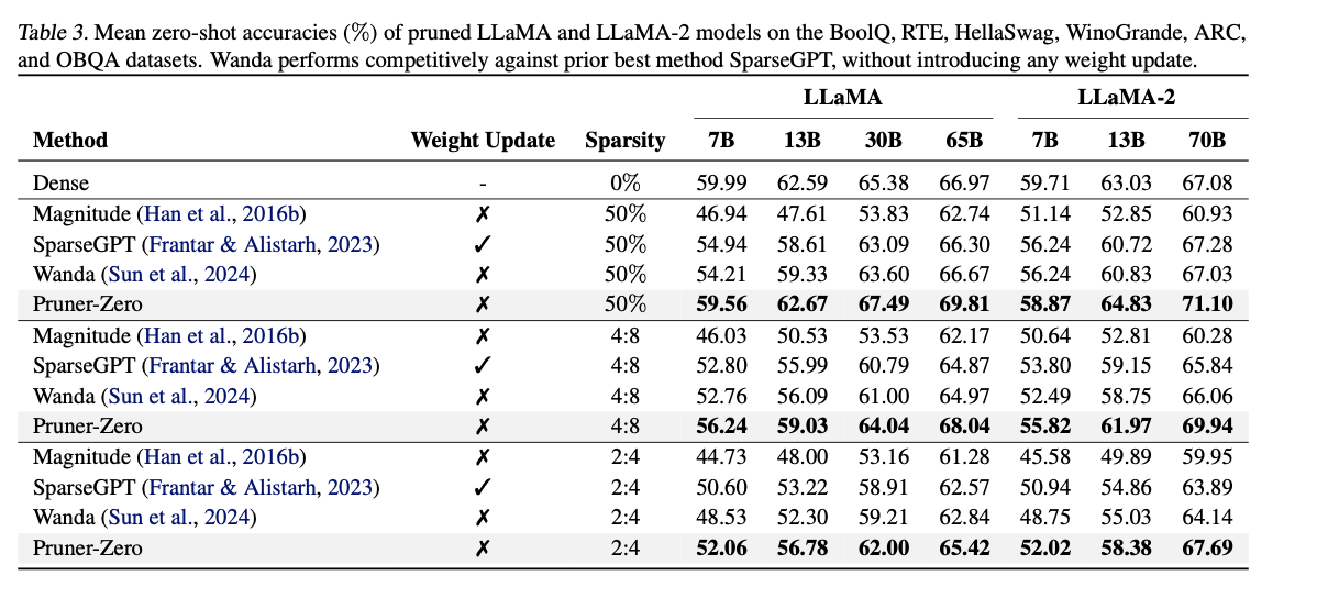
Research on inverting Neural Radiance Fields makes a substantial contribution to the field of AI by addressing the challenge of 3D scene reconstruction from 2D images. The new approach leverages a novel optimization framework and a latent feature space to invert NeRFs, providing a more efficient and accurate solution compared to existing methods. The findings demonstrate significant improvements in reconstruction accuracy and computational efficiency, highlighting the potential impact of this work on applications in AR, VR, and robotic perception. By overcoming a critical challenge in 3D scene understanding, this research advances the field of AI and opens new avenues for future exploration and development.
Check out the Paper and GitHub . All credit for this research goes to the researchers of this project. Also, don’t forget to follow us on Twitter .
Join our Telegram Channel and LinkedIn Gr oup .
If you like our work, you will love our newsletter..
Don’t Forget to join our 45k+ ML SubReddit

Aswin AK is a consulting intern at MarkTechPost. He is pursuing his Dual Degree at the Indian Institute of Technology, Kharagpur. He is passionate about data science and machine learning, bringing a strong academic background and hands-on experience in solving real-life cross-domain challenges.
- Cutting Costs, Not Performance: Structured FeedForward Networks FFNs in Transformer-Based LLMs
- A Comprehensive Overview of Prompt Engineering for ChatGPT
- A Deep Dive into Group Relative Policy Optimization (GRPO) Method: Enhancing Mathematical Reasoning in Open Language Models
- This AI Paper from Google DeepMind Explores the Effect of Communication Connectivity in Multi-Agent Systems
RELATED ARTICLES MORE FROM AUTHOR
Fal ai introduces aurasr: a 600m parameter upsampler model derived from the gigagan, arcee ai release arcee spark: a new era of compact and efficient 7b parameter language models, wildteaming: an automatic red-team framework to compose human-like adversarial attacks using diverse jailbreak tactics devised by creative and self-motivated users in-the-wild, claude engineer: an interactive command-line interface (cli) that leverages the power of anthropic’s claude-3.5-sonnet model to assist with software development tasks, ragapp: an ai starter kit to build your own agentic rag in the enterprise as simple as using gpts, math-llava: a llava-1.5-based ai model fine-tuned with mathv360k dataset, arcee ai release arcee spark: a new era of compact and efficient 7b parameter..., wildteaming: an automatic red-team framework to compose human-like adversarial attacks using diverse jailbreak tactics..., claude engineer: an interactive command-line interface (cli) that leverages the power of anthropic’s claude-3.5-sonnet..., ragapp: an ai starter kit to build your own agentic rag in the enterprise....
- AI Magazine
- Privacy & TC
- Cookie Policy
🐝 🐝 Join the Fastest Growing AI Research Newsletter...
Thank You 🙌
Privacy Overview
Mashee at SemEval-2024 Task 8: The Impact of Samples Quality on the Performance of In-Context Learning for Machine Text Classification
Within few-shot learning, in-context learning (ICL) has become a potential method for leveraging contextual information to improve model performance on small amounts of data or in resource-constrained environments where training models on large datasets is prohibitive. However, the quality of the selected sample in a few shots severely limits the usefulness of ICL. The primary goal of this paper is to enhance the performance of evaluation metrics for in-context learning by selecting high-quality samples in few-shot learning scenarios. We employ the chi-square test to identify high-quality samples and compare the results with those obtained using low-quality samples. Our findings demonstrate that utilizing high-quality samples leads to improved performance with respect to all evaluated metrics.
1 Introduction
The advent of large language models (LLMs) like GPT-3.5 has brought about transformative capabilities, seamlessly handling tasks like question answering, essay writing, and problem-solving Aljanabi et al. ( 2023 ); Wu et al. ( 2023 ); Rasheed et al. ( 2023a ) . However, this technological advancement necessitates careful consideration of its associated challenges. Concerns regarding the potential impact on creativity and ethical implications, particularly concerning the generation of deepfakes Tang et al. ( 2023 ) , warrant careful attention RAYMOND ( 2023 ) . Additionally, the limitations of LLMs, including the possibility of producing erroneous information, require rigorous evaluation and verification. The substantial energy consumption required for training LLMs on massive datasets raises environmental concerns, contributing to their carbon footprint. Moreover, plagiarism issues emerge as users may misuse the generated content, either inadvertently or intentionally Hadi et al. ( 2023 ) .
Various models have been introduced in recent years designed to distinguish text generated by humans from that created by machines Mitchell et al. ( 2023 ) . Examples include GPTZero gpt , AI Content Detector cop , and AI Content Detector by Writer wri among others. Some of these models are trained on specific datasets, while others are commercially available. Designing and implementing LLMs for classification tasks requires substantial resources and computational power, which are often only accessible to institutions and governments. Therefore, various optimization models, such as LoRA Hu et al. ( 2021 ) , distillation Hsieh et al. ( 2023 ) , quantization Dettmers et al. ( 2022 ) , and in-context learning Liu et al. ( 2022 ) , have been developed to reduce the resource requirements for LLM implementation. This paper focuses on In Context Learning (ICL) Liu et al. ( 2022 ) , which utilizes the capabilities of other models to enhance their ability to classify AI-generated text.
In Context Learning (ICL) is a Natural Language Processing (NLP) technique utilized to enable Large Language Models (LLMs) to learn new tasks based on minimal examples. This technique proves powerful in scenarios where training models on extensive datasets is impractical or when there are constraints on dataset availability for a specific task. ICL operates on the premise that humans can often acquire new tasks through analogy or by observing a few examples of task performance. It can be employed without any examples and is referred to as zero-shot learning. Alternatively, if the input includes one example, it is termed one-shot learning, and if it contains more than one, it is known as few-shot learning. This paper focuses on the application of few-shot learning within the context of ICL Ahmed and Devanbu ( 2022 ); Kang et al. ( 2023 ) .
In this study, our focus lies exclusively on few-shot learning. We present a methodology that leverages the chi-square statistic Rasheed et al. ( 2023b ); Lancaster and Seneta ( 2005 ) to select samples for few-shot learning and evaluate its impact on the performance of a machine-generated text classification model. We work on task A English language only Wang et al. ( 2024 ) .
The dataset employed for Task A comprises two main components. The first part, derived from human writing, was collected from diverse sources including WikiBidia, WikiHow, Reddit, ArXiv, and PeerRead. The second part consists of a machine-generated text produced by ChatGPT, Cohere, Dolly-v2, and BLOOMz Muennighoff et al. ( 2023 ) . For further details, please refer to the associated paper Wang et al. ( 2023 ) .
3 Chi-square
Chi-square is a statistical test used to assess the independence of two categorical variables. It calculates the difference between observed and expected frequencies of outcomes, and a larger chi-square value indicates a stronger rejection of independence. In text analysis, chi-square can be used to identify keywords that are more likely to occur in one category than another, making it useful for feature selection and text classification. We computed the chi-square values for each training sample and recorded the sample index with the highest and lowest chi-square values for both human-generated and machine-generated samples. Table I displays the index and corresponding chi-square values for each of these instances. We will use X 2 superscript 𝑋 2 X^{2} italic_X start_POSTSUPERSCRIPT 2 end_POSTSUPERSCRIPT to refer to chi-square Lancaster and Seneta ( 2005 ) .
| Name | Index # | Value |
|---|---|---|
| Highest (Human) | 70873 | 1351.59 |
| Lowest (Human) | 85726 | 1.21 |
| Highest (Machine) | 2426 | 1154.27 |
| Lowest (Machine) | 29111 | 0.8243 |
4 System overview

The system architecture is illustrated in Figure 1. The process starts with feeding the entire training dataset to a chi-square computation, where the chi-square value for each sample is calculated. Subsequently, the indices of the samples with the highest and lowest chi-square values are selected for both human-generated and machine-generated datasets using information from Table I. Next, context learning is prepared. Initially, multiple templates were tested, and the one presented in Figure 1 yielded the best results. This template is then fed with two samples: the first being the machine-generated sample with the highest chi-square value, and the second being the human-generated sample with the highest chi-square value. Due to context window size limitations, only the first 5000 characters of each sample are incorporated. This is applied to training samples exceeding 5000 characters to ensure the context learning size is not exceeded. Finally, the test sample is fed into the context-learning process. The Flan-T5 model large version is used. The results are then recorded and evaluated. The dev/test sample size was truncated to 3000. We also evaluated the system using samples with the lowest chi-square values and doing the same process.
| Dataset | Chi Type | Recall | Precision | F1-Score | Accuracy |
|---|---|---|---|---|---|
| Dev set | Lowest | 46.92 | 46.90 | 46.84 | 46.92 |
| Highest | 53.76 | 53.76 | 53.74 | 53.76 | |
| Test set | Lowest | 55.04 | 55.07 | 55.03 | 55.27 |
| Highest | 58.68 | 58.81 | 58.81 | 55.99 |
5 Findings and Analysis
We employed the Flan-T5 Large model for both the development and testing datasets. We selected samples from both human-generated and machine-generated sources, with each sample limited to 5000 characters to avoid exceeding the token size limit. A total of four experiments were conducted. The first experiment utilized samples with high chi-square values from the development set. The second experiment focused on samples with the smallest chi-square values from the development set. The third experiment involved samples with high chi-square values from the test set. Finally, the fourth experiment utilized samples with low chi-square values from the test set. Table II presents all achieved results.
Based on the results presented in Table II, we can discuss several key points.
The results highlight the crucial role of sample quality in the performance of in-context learning. By leveraging the chi-squared metric and prioritizing samples with high values, we essentially provide the Flan-T5 model with examples rich in diverse features. This choice enables the Flan-T5 model to learn more effectively, drawing substantial insights from the samples. Consequently, the model becomes more familiar with the provided data, ultimately enhancing its performance. In contrast, selecting samples with lower quality leads to less optimal performance. This can be noticed for both the dev and test set. The main reason behind this is that words in the sample with high chi-square values contain the most distinctive features. This is because the chi-square test assigns high values to words that are frequent within a particular class but appear less frequently in other classes.Conversely, samples with lower chi-square values likely contain more random words that appear with similar frequency across all classes. In chi-square analysis, words that appear equally or approximately equally in each class receive lower scores.
The classification of machine-generated text represents a novel frontier in machine learning, and the availability of datasets for this task is currently limited. The dataset used in this study was generated in 2023, marking it as a recent development and underscoring the lack of established benchmarks. Models that support in-context learning have not been trained extensively on such tasks, resulting in lower accuracy when applied. While examples with high-quality data can enhance model performance, it remain below the desired threshold. Hence, it is advisable to train the model directly on the dataset rather than relying on in-context learning.
We have utilized the Flan-T5 model; however, other models can be employed to evaluate the performance of text classification machinery. We suggest considering alternatives such as bard, Jurassic-1 Jumbo, and ChatGPT.
6 Conclusion
This work presents a system for classifying human-generated and machine-generated text. The system leverages the combined strengths of in-context learning and Chi-square analysis. Chi-square is employed to select high-quality samples from the trainin dataset for few-shot learning in the in-context learning. We implement Flan-T5 model large version for in-context learning. Evaluation using accuracy, recall, precision, and F1-score demonstrates that selecting high-quality samples improves system performance for both dev and test. Furthermore, the results indicate that relying solely on in-context learning for new tasks like machine-generated text detection yields relatively low performance.
- (1) Ai content detector . Accessed on May 28, 2024.
- (2) Ai content detector by writer . Accessed on May 28, 2024.
- (3) Gptzero . Accessed on May 28, 2024.
- Ahmed and Devanbu (2022) Toufique Ahmed and Premkumar Devanbu. 2022. Few-shot training llms for project-specific code-summarization. In Proceedings of the 37th IEEE/ACM International Conference on Automated Software Engineering , pages 1–5.
- Aljanabi et al. (2023) Mohammad Aljanabi, Mohanad Ghazi, Ahmed Hussein Ali, Saad Abas Abed, et al. 2023. Chatgpt: open possibilities. Iraqi Journal For Computer Science and Mathematics , 4(1):62–64.
- Dettmers et al. (2022) Tim Dettmers, Mike Lewis, Younes Belkada, and Luke Zettlemoyer. 2022. Llm. int8 (): 8-bit matrix multiplication for transformers at scale. arXiv preprint arXiv:2208.07339 .
- Hadi et al. (2023) Muhammad Usman Hadi, R Qureshi, A Shah, M Irfan, A Zafar, MB Shaikh, N Akhtar, J Wu, and S Mirjalili. 2023. A survey on large language models: Applications, challenges, limitations, and practical usage. TechRxiv .
- Hsieh et al. (2023) Cheng-Yu Hsieh, Chun-Liang Li, Chih-Kuan Yeh, Hootan Nakhost, Yasuhisa Fujii, Alexander Ratner, Ranjay Krishna, Chen-Yu Lee, and Tomas Pfister. 2023. Distilling step-by-step! outperforming larger language models with less training data and smaller model sizes. arXiv preprint arXiv:2305.02301 .
- Hu et al. (2021) Edward J. Hu, Yelong Shen, Phillip Wallis, Zeyuan Allen-Zhu, Yuanzhi Li, Shean Wang, Lu Wang, and Weizhu Chen. 2021. Lora: Low-rank adaptation of large language models .
- Kang et al. (2023) Sungmin Kang, Juyeon Yoon, and Shin Yoo. 2023. Large language models are few-shot testers: Exploring llm-based general bug reproduction. In 2023 IEEE/ACM 45th International Conference on Software Engineering (ICSE) , pages 2312–2323. IEEE.
- Lancaster and Seneta (2005) Henry Oliver Lancaster and Eugene Seneta. 2005. Chi-square distribution. Encyclopedia of biostatistics , 2.
- Liu et al. (2022) Haokun Liu, Derek Tam, Mohammed Muqeeth, Jay Mohta, Tenghao Huang, Mohit Bansal, and Colin A Raffel. 2022. Few-shot parameter-efficient fine-tuning is better and cheaper than in-context learning. Advances in Neural Information Processing Systems , 35:1950–1965.
- Mitchell et al. (2023) Eric Mitchell, Yoonho Lee, Alexander Khazatsky, Christopher D Manning, and Chelsea Finn. 2023. Detectgpt: Zero-shot machine-generated text detection using probability curvature. arXiv preprint arXiv:2301.11305 .
- Muennighoff et al. (2023) Niklas Muennighoff, Thomas Wang, Lintang Sutawika, Adam Roberts, Stella Biderman, Teven Le Scao, M Saiful Bari, Sheng Shen, Zheng-Xin Yong, Hailey Schoelkopf, Xiangru Tang, Dragomir Radev, Alham Fikri Aji, Khalid Almubarak, Samuel Albanie, Zaid Alyafeai, Albert Webson, Edward Raff, and Colin Raffel. 2023. Crosslingual generalization through multitask finetuning .
- Rasheed et al. (2023a) Areeg Fahad Rasheed, M Zarkoosh, Safa F Abbas, and Sana Sabah Al-Azzawi. 2023a. Arabic offensive language classification: Leveraging transformer, lstm, and svm. In 2023 IEEE International Conference on Machine Learning and Applied Network Technologies (ICMLANT) , pages 1–6. IEEE.
- Rasheed et al. (2023b) Areeg Fahad Rasheed, M Zarkoosh, and Sana Sabah Al-Azzawi. 2023b. The impact of feature selection on malware classification using chi-square and machine learning. In 2023 9th International Conference on Computer and Communication Engineering (ICCCE) , pages 211–216. IEEE.
- RAYMOND (2023) DANIEL RAYMOND. 2023. Disadvantages of large language models . Accessed on May 28, 2024.
- Tang et al. (2023) Ruixiang Tang, Yu-Neng Chuang, and Xia Hu. 2023. The science of detecting llm-generated texts. arXiv preprint arXiv:2303.07205 .
- Wang et al. (2023) Yuxia Wang, Jonibek Mansurov, Petar Ivanov, Jinyan Su, Artem Shelmanov, Akim Tsvigun, Chenxi Whitehouse, Osama Mohammed Afzal, Tarek Mahmoud, Alham Fikri Aji, and Preslav Nakov. 2023. M4: Multi-generator, multi-domain, and multi-lingual black-box machine-generated text detection .
- Wang et al. (2024) Yuxia Wang, Jonibek Mansurov, Petar Ivanov, Jinyan Su, Artem Shelmanov, Akim Tsvigun, Chenxi Whitehouse, Osama Mohammed Afzal, Tarek Mahmoud, Giovanni Puccetti, Thomas Arnold, Alham Fikri Aji, Nizar Habash, Iryna Gurevych, and Preslav Nakov. 2024. SemEval-2024 task 8: Multigenerator, multidomain, and multilingual black-box machine-generated text detection. In Proceedings of the 18th International Workshop on Semantic Evaluation , SemEval 2024, Mexico City, Mexico.
- Wu et al. (2023) Tianyu Wu, Shizhu He, Jingping Liu, Siqi Sun, Kang Liu, Qing-Long Han, and Yang Tang. 2023. A brief overview of chatgpt: The history, status quo and potential future development. IEEE/CAA Journal of Automatica Sinica , 10(5):1122–1136.
- Professional
- International
Select a product below:
- Connect Math Hosted by ALEKS
- My Bookshelf (eBook Access)
Sign in to Shop:
My Account Details
- My Information
- Security & Login
- Order History
Log In to My PreK-12 Platform
- AP/Honors & Electives
- my.mheducation.com
- Open Learning Platform
Log In to My Higher Ed Platform
- Connect Math Hosted by Aleks
Business and Economics
Accounting Business Communication Business Law Business Mathematics Business Statistics & Analytics Computer & Information Technology Decision Sciences & Operations Management Economics Finance Keyboarding Introduction to Business Insurance & Real Estate Management Information Systems Management Marketing
Humanities, Social Science and Language
American Government Anthropology Art Career Development Communication Criminal Justice Developmental English Education Film Composition Health and Human Performance
History Humanities Music Philosophy and Religion Psychology Sociology Student Success Theater World Languages
Science, Engineering and Math
Agriculture & Forestry Anatomy & Physiology Astronomy & Physical Science Biology - Majors Biology - Non-Majors Chemistry Cell/Molecular Biology & Genetics Earth & Environmental Science Ecology Engineering/Computer Science Engineering Technologies - Trade & Tech Health Professions Mathematics Microbiology Nutrition Physics Plants & Animals
Digital Products
Connect® Course management , reporting , and student learning tools backed by great support .
McGraw Hill GO Greenlight learning with the new eBook+
ALEKS® Personalize learning and assessment
ALEKS® Placement, Preparation, and Learning Achieve accurate math placement
SIMnet Ignite mastery of MS Office and IT skills
McGraw Hill eBook & ReadAnywhere App Get learning that fits anytime, anywhere
Sharpen: Study App A reliable study app for students
Virtual Labs Flexible, realistic science simulations
Inclusive Access Reduce costs and increase success
LMS Integration Log in and sync up
Math Placement Achieve accurate math placement
Content Collections powered by Create® Curate and deliver your ideal content
Custom Courseware Solutions Teach your course your way
Professional Services Collaborate to optimize outcomes
Remote Proctoring Validate online exams even offsite
Institutional Solutions Increase engagement, lower costs, and improve access for your students
General Help & Support Info Customer Service & Tech Support contact information
Online Technical Support Center FAQs, articles, chat, email or phone support
Support At Every Step Instructor tools, training and resources for ALEKS , Connect & SIMnet
Instructor Sample Requests Get step by step instructions for requesting an evaluation, exam, or desk copy
Platform System Check System status in real time
Understanding AI Bias (and How to Address It) | January 2024
Ai is machine learning that can perform activities and tasks that usually require human intelligence such as decisions, visual perception, and speech recognition..

Artificial intelligence (AI) relates to machine learning that is able to perform activities and tasks that usually require human intelligence such as decisions, visual perception, and speech recognition. AI bias, which refers to the systematic prejudices within algorithms that result in unfair outcomes or discrimination against certain groups, is an important business ethics issue. These biases can significantly impact decision-making processes, perpetuating societal inequalities.
Causes of AI Bias
A significant source of AI bias is biased data. Machine learning models learn from historical data and programming, inheriting any biases present within it. If the training data is skewed or unrepresentative, the model can perpetuate existing biases. For example, if a company trains an AI recruitment tool with historical data that favors male applicants, then the algorithms will continue to favor male applicants. In one example, Amazon had to scrap a recruiting engine it developed after discovering it showed bias against women.
Algorithmic design choices also contribute to bias. Decisions made during algorithm development by humans, such as feature selection or model architecture, can amplify biases present in the data, further influencing outcomes.
Additionally, a lack of diversity in development teams can inadvertently lead to overlooked biases. The technology sector has a major diversity problem. Diverse perspectives and experiences are crucial in identifying and addressing potential biases within AI systems. This is one of the many reasons why diversity is important in business.
Another critical factor is the implicit biases of the developers themselves. AI models are made by people, after all. Unconscious biases can seep into the AI systems during their creation, affecting decision-making processes and outcomes.
Avoiding AI Bias
There are several strategies to avoid AI bias, but diversity in applications and algorithms makes it impossible to find one clear path. Using diverse and representative data sets is fundamental. Carefully curated datasets that account for various demographics can significantly reduce bias.
Continuous audits and testing of AI systems are essential. Regular monitoring helps detect biases, and rigorous testing against diverse scenarios allows for the identification and rectification of potential biases before deployment. OpenAI , the company behind chatbot ChatGPT, trains models with large datasets from the internet, trains them again with a narrower dataset curated by human reviewers following set guidelines, and fine-tunes the model by keeping feedback channels open.
Additionally, transparency and accountability are vital. AI systems should be transparent in their decision-making processes, providing explanations that enable understanding of why certain decisions are made. This facilitates bias identification and corrective action. Companies should also be held accountable for the AI models they develop.
Encouraging diversity within development teams is also pivotal. Diverse teams bring different perspectives, aiding in identifying and mitigating biases effectively.
Ethical Implications
The ethical implications of AI bias are of great concern. Biased AI systems can perpetuate discrimination and unfairness, affecting opportunities in areas such as employment, finance, and healthcare. Lack of accountability in biased AI decision-making processes poses challenges in taking corrective action.
Moreover, these systems can inadvertently reinforce societal stereotypes, deepening social divides and hindering progress toward a more equitable society. Legal and regulatory concerns regarding the accountability and fairness of AI systems further underscore the urgency of addressing bias.
Tackling AI bias requires concerted efforts in data collection, algorithmic design, diversity in development, and adherence to ethical guidelines. Through these strategies, it's possible to mitigate bias and ensure AI systems promote fairness, inclusivity, and ethical decision-making.
In the Classroom
This article can be used to discuss business ethics (Chapter 2: Business Ethics and Social Responsibility).
Discussion Questions
- What is AI bias?
- What factors can contribute to AI bias?
- How can AI bias be reduced (or eliminated)?
This article was developed with the support of Kelsey Reddick for and under the direction of O.C. Ferrell, Linda Ferrell, and Geoff Hirt.
Cheyenne DeVon, "How to Reduce AI Bias, According to Tech Expert," CNBC, December 16, 2023, https://www.cnbc.com/2023/12/16/how-to-reduce-ai-bias-according-to-tech-expert.html?__source=iosappshare%7Ccom.apple.UIKit.activity.Mail
Michael Li, "To Build Less-Biased AI, Hire a More-Diverse Team," Harvard Business Review, October 26, 2020, https://hbr.org/2020/10/to-build-less-biased-ai-hire-a-more-diverse-team
Monika Mueller, "The Ethics Of AI: Navigating Bias, Manipulation and Beyond," Forbes, June 23, 2023, https://www.forbes.com/sites/forbestechcouncil/2023/06/23/the-ethics-of-ai-navigating-bias-manipulation-and-beyond/?sh=5015c85e40a2
Author: OC Ferrell O.C. Ferrell is the James T. Pursell Sr. Eminent Scholar in Ethics and Director of the Center for Ethical Organizational Cultures in the Raymond J. Harbert College of Business, Auburn University. He was formerly Distinguished Professor of Leadership and Business Ethics at Belmont University and University Distinguished Professor at the University of New Mexico. He has also been on the faculties of the University of Wyoming, Colorado State University, University of Memphis, Texas A&M University, Illinois State University, and Southern Illinois University. He received his Ph.D. in marketing from Louisiana State University.
IMAGES
VIDEO
COMMENTS
A machine learning task is the type of prediction or inference being made, based on the problem or question that is being asked, and the available data. For example, the classification task assigns data to categories, and the clustering task groups data according to similarity. Machine learning tasks rely on patterns in the data rather than ...
Examples include: Email spam detection (spam or not). Churn prediction (churn or not). Conversion prediction (buy or not). Typically, binary classification tasks involve one class that is the normal state and another class that is the abnormal state. For example " not spam " is the normal state and " spam " is the abnormal state.
scikit-learn #. One of the most prominent Python libraries for machine learning: Contains many state-of-the-art machine learning algorithms. Builds on numpy (fast), implements advanced techniques. Wide range of evaluation measures and techniques. Offers comprehensive documentation about each algorithm.
After completing each unit, there will be a 20 minute quiz (taken online via gradescope). Each quiz will be designed to assess your conceptual understanding about each unit. Probably 10 questions. Most questions will be true/false or multiple choice, with perhaps 1-3 short answer questions. You can view the conceptual questions in each unit's ...
Machine learning is about learning some properties of a data set and then testing those properties against another data set. A common practice in machine learning is to evaluate an algorithm by splitting a data set into two. We call one of those sets the training set, on which we learn some properties; we call the other set the testing set, on ...
Artificial Intelligence (AI) is a broad term used to describe systems capable of making certain decisions on their own. Machine Learning (ML) is a specific subject within the broader AI arena, describing the ability for a machine to improve its ability by practicing a task or being exposed to large data sets.
-Select the appropriate machine learning task for a potential application. -Apply regression, classification, clustering, retrieval, recommender systems, and deep learning. ... Access to lectures and assignments depends on your type of enrollment. If you take a course in audit mode, you will be able to see most course materials for free. ...
In this step-by-step tutorial you will: Download and install Python SciPy and get the most useful package for machine learning in Python. Load a dataset and understand it's structure using statistical summaries and data visualization. Create 6 machine learning models, pick the best and build confidence that the accuracy is reliable.
As a Machine Learning Researcher or Machine Learning Engineer, there are many technical tools and programming languages you might use in your day-to-day job. But for today and for this handbook, we'll use the programming language and tools: Python Basics: Variables, data types, structures, and control mechanisms.
This repository contains the exercises, lab works and home works assignment for the Introduction to Machine Learning online class taught by Professor Leslie Pack Kaelbling, Professor Tomás Lozano-Pérez, Professor Isaac L. Chuang and Professor Duane S. Boning from Massachusett Institute of Technology - denikn/Machine-Learning-MIT-Assignment
Image by Author Feature Engineering. We need to transform the data before we build the model. We will use a data manipulation technique called feature engineering to transform the data. Feature engineering refers to the manipulation of a dataset (addition, deletion, combination, etc) to improve machine learning model training, leading to better performance, and greater accuracy.
Machine learning (ML) is a subdomain of artificial intelligence (AI) that focuses on developing systems that learn—or improve performance—based on the data they ingest. Artificial intelligence is a broad word that refers to systems or machines that resemble human intelligence. Machine learning and AI are frequently discussed together, and ...
Conclusion. That covers the basics of the three core types of machine learning: classification, regression, and clustering. As you get started with machine learning, I strongly encourage you to start with classification or regression. In fact, a standard experiment for new data scientists is to start out with a binary classification experiment ...
If the machine learning models do not beat this guess, then we might have to conclude that machine learning is not acceptable for the task or we might need to try a different approach. For regression problems, a reasonable naive baseline is to guess the median value of the target on the training set for all the examples in the test set.
-Build machine learning models in Python using popular machine learning libraries NumPy and scikit-learn. Build and train supervised machine learning models for prediction and binary classification tasks, including linear regression and logistic regression. Build and train a neural network with TensorFlow to perform multi-class classification.
Contains Optional Labs and Solutions of Programming Assignment for the Machine Learning Specialization By Stanford University and Deeplearning.ai - Coursera (2023) by Prof. Andrew NG - A-sad-ali/Machine-Learning-Specialization ... Build and train supervised machine learning models for prediction and binary classification tasks, including linear ...
20. MLOps End-To-End Machine Learning. The MLOps End-To-End Machine Learning project is necessary for you to get hired by top companies. Nowadays, recruiters are looking for ML engineers who can create end-to-end systems using MLOps tools, data orchestration, and cloud computing.
Download scientific diagram | Task Assignment algorithm following the machine learning approach from publication: Job Aware Scheduling Algorithm for MapReduce Framework | MapReduce framework has ...
We argue that viewing multi-target tracking as an assignment problem conceptually unifies the wide variety of machine learning methods that have been proposed for data association and track-to-track association. In this survey, we review recent literature, provide rigorous formulations of the assignment problems encountered in multi-target ...
View PDF Abstract: We present an end-to-end framework for the Assignment Problem with multiple tasks mapped to a group of workers, using reinforcement learning while preserving many constraints. Tasks and workers have time constraints and there is a cost associated with assigning a worker to a task. Each worker can perform multiple tasks until it exhausts its allowed time units (capacity).
Although research on human-machine task assignment has presently received academic attention, the theoretical foundation of task assignment requires further development. ... Machine learning is ...
We present Reinforcement Learning via Auxiliary Task Distillation (AuxDistill), a new method that enables reinforcement learning (RL) to perform long-horizon robot control problems by distilling behaviors from auxiliary RL tasks. AuxDistill achieves this by concurrently carrying out multi-task RL with auxiliary tasks, which are easier to learn and relevant to the main task. A weighted ...
The model's task is to match the X-ray with its correct report. Mathematically, the model does this by learning how to store the matching image and report closer to each other, with the unmatched image and report farther away from each other in the models' learning space, referred to as its representation space (Figure 3). Simply explained ...
There will be one homework (HW) for each topical unit of the course, due soon after we finish that unit. These are intended to build your conceptual analysis skills plus your implementation skills in Python. HW0: Numerical Programming Fundamentals. HW1: Regression, Cross-Validation, and Regularization. HW2: Evaluating Binary Classifiers and ...
NinjaTech AI's mission is to make everyone more productive by taking care of time-consuming complex tasks with fast and affordable artificial intelligence (AI) agents. We recently launched MyNinja.ai, one of the world's first multi-agent personal AI assistants, to drive towards our mission. MyNinja.ai is built from the ground up using specialized agents that are capable of completing tasks ...
This is the official repository contains complete code of Machine Learning training provided by internshala. Topics internshala internshalaassignment internshala-finalproject internshala-machine-learning internshalatraining
Also, implementing these technologies would create significant time savings, freeing up extra time and manpower for training and readiness tasks. Conclusion. Senior leaders across the Department of Defense and Marine Corps have stated that AI and machine learning are the way forward for the future force. The efficiency loss created by the ...
A major challenge in computer vision and graphics is the ability to reconstruct 3D scenes from sparse 2D images. Traditional Neural Radiance Fields (NeRFs), while effective for rendering photorealistic views from novel perspectives, are inherently limited to forward rendering tasks and cannot invert to deduce the 3D structure from 2D projections. This limitation hinders the broader ...
The classification of machine-generated text represents a novel frontier in machine learning, and the availability of datasets for this task is currently limited. The dataset used in this study was generated in 2023, marking it as a recent development and underscoring the lack of established benchmarks.
AI is machine learning that can perform activities and tasks that usually require human intelligence such as decisions, visual perception, and speech recognition. January 12, 2024. Article Artificial Intelligence (AI) Blog Ferrell Business in the News Higher Education.