homework 3 writing linear equations applications & linear regression

12.3 The Regression Equation

Data rarely fit a straight line exactly. Usually, you must be satisfied with rough predictions. Typically, you have a set of data whose scatter plot appears to "fit" a straight line. This is called a Line of Best Fit or Least-Squares Line .

Collaborative Exercise

If you know a person's pinky (smallest) finger length, do you think you could predict that person's height? Collect data from your class (pinky finger length, in inches). The independent variable, x , is pinky finger length and the dependent variable, y , is height. For each set of data, plot the points on graph paper. Make your graph big enough and use a ruler . Then "by eye" draw a line that appears to "fit" the data. For your line, pick two convenient points and use them to find the slope of the line. Find the y -intercept of the line by extending your line so it crosses the y -axis. Using the slopes and the y -intercepts, write your equation of "best fit." Do you think everyone will have the same equation? Why or why not? According to your equation, what is the predicted height for a pinky length of 2.5 inches?

Example 12.6

A random sample of 11 statistics students produced the following data, where x is the third exam score out of 80, and y is the final exam score out of 200. Can you predict the final exam score of a random student if you know the third exam score?

Try It 12.6

SCUBA divers have maximum dive times they cannot exceed when going to different depths. The data in Table 12.4 show different depths with the maximum dive times in minutes. Use your calculator to find the least squares regression line and predict the maximum dive time for 110 feet.

The third exam score, x , is the independent variable and the final exam score, y , is the dependent variable. We will plot a regression line that best "fits" the data. If each of you were to fit a line "by eye," you would draw different lines. We can use what is called a least-squares regression line to obtain the best fit line.

Consider the following diagram. Each point of data is of the the form ( x , y ) and each point of the line of best fit using least-squares linear regression has the form ( x , ŷ ).

The ŷ is read " y hat" and is the estimated value of y . It is the value of y obtained using the regression line. It is not generally equal to y from data.

The term y 0 – ŷ 0 = ε 0 is called the "error" or residual . It is not an error in the sense of a mistake. The absolute value of a residual measures the vertical distance between the actual value of y and the estimated value of y . In other words, it measures the vertical distance between the actual data point and the predicted point on the line.

If the observed data point lies above the line, the residual is positive, and the line underestimates the actual data value for y . If the observed data point lies below the line, the residual is negative, and the line overestimates that actual data value for y .

In the diagram in Figure 12.10 , y 0 – ŷ 0 = ε 0 is the residual for the point shown. Here the point lies above the line and the residual is positive.

ε = the Greek letter epsilon

For each data point, you can calculate the residuals or errors, y i - ŷ i = ε i for i = 1, 2, 3, ..., 11.

Each | ε | is a vertical distance.

For the example about the third exam scores and the final exam scores for the 11 statistics students, there are 11 data points. Therefore, there are 11 ε values. If you square each ε and add, you get

This is called the Sum of Squared Errors (SSE) .

Using calculus, you can determine the values of a and b that make the SSE a minimum. When you make the SSE a minimum, you have determined the points that are on the line of best fit. It turns out that the line of best fit has the equation:

where a = y ¯ − b x ¯ a = y ¯ − b x ¯ and b = Σ ( x − x ¯ ) ( y − y ¯ ) Σ ( x − x ¯ ) 2 b = Σ ( x − x ¯ ) ( y − y ¯ ) Σ ( x − x ¯ ) 2 .

The sample means of the x values and the y values are x ¯ x ¯ and y ¯ y ¯ , respectively. The best fit line always passes through the point ( x ¯ , y ¯ ) ( x ¯ , y ¯ ) .

The slope b can be written as b = r ( s y s x ) b = r ( s y s x ) where s y = the standard deviation of the y values and s x = the standard deviation of the x values. r is the correlation coefficient, which is discussed in the next section.

Residuals Plots

A residuals plot can be used to help determine if a set of ( x , y ) data is linearly correlated. For each data point used to create the correlation line, a residual y - y can be calculated, where y is the observed value of the response variable and y is the value predicted by the correlation line. The difference between these values is called the residual. A residuals plot shows the explanatory variable x on the horizontal axis and the residual for that value on the vertical axis. The residuals plot is often shown together with a scatter plot of the data. While a scatter plot of the data should resemble a straight line, a residuals plot should appear random, with no pattern and no outliers. It should also show constant error variance, meaning the residuals should not consistently increase (or decrease) as the explanatory variable x increases.

A residuals plot can be created using StatCrunch or a TI calculator. The plot should appear random. A box plot of the residuals is also helpful to verify that there are no outliers in the data. By observing the scatter plot of the data, the residuals plot, and the box plot of residuals, together with the linear correlation coefficient, we can usually determine if it is reasonable to conclude that the data are linearly correlated.

A shop owner uses a straight-line regression to estimate the number of ice cream cones that would be sold in a day based on the temperature at noon. The owner has data for a 2-year period and chose nine days at random. A scatter plot of the data is shown, together with a residuals plot.

Least Squares Criteria for Best Fit

The process of fitting the best-fit line is called linear regression . The idea behind finding the best-fit line is based on the assumption that the data are scattered about a straight line. The criteria for the best fit line is that the sum of the squared errors (SSE) is minimized, that is, made as small as possible. Any other line you might choose would have a higher SSE than the best fit line. This best fit line is called the least-squares regression line .

Computer spreadsheets, statistical software, and many calculators can quickly calculate the best-fit line and create the graphs. The calculations tend to be tedious if done by hand. Instructions to use the TI-83, TI-83+, and TI-84+ calculators to find the best-fit line and create a scatterplot are shown at the end of this section.

THIRD EXAM vs FINAL EXAM EXAMPLE: The graph of the line of best fit for the third-exam/final-exam example is as follows:

The least squares regression line (best-fit line) for the third-exam/final-exam example has the equation:

Remember, it is always important to plot a scatter diagram first. If the scatter plot indicates that there is a linear relationship between the variables, then it is reasonable to use a best fit line to make predictions for y given x within the domain of x -values in the sample data, but not necessarily for x -values outside that domain. You could use the line to predict the final exam score for a student who earned a grade of 73 on the third exam. You should NOT use the line to predict the final exam score for a student who earned a grade of 50 on the third exam, because 50 is not within the domain of the x -values in the sample data, which are between 65 and 75.

UNDERSTANDING SLOPE

The slope of the line, b , describes how changes in the variables are related. It is important to interpret the slope of the line in the context of the situation represented by the data. You should be able to write a sentence interpreting the slope in plain English.

INTERPRETATION OF THE SLOPE: The slope of the best-fit line tells us how the dependent variable ( y ) changes for every one unit increase in the independent ( x ) variable, on average.

THIRD EXAM vs FINAL EXAM EXAMPLE Slope: The slope of the line is b = 4.83. Interpretation: For a one-point increase in the score on the third exam, the final exam score increases by 4.83 points, on average.

Using the TI-83, 83+, 84, 84+ Calculator

Using the Linear Regression T Test: LinRegTTest

• In the STAT list editor, enter the X data in list L1 and the Y data in list L2 , paired so that the corresponding ( x , y ) values are next to each other in the lists. (If a particular pair of values is repeated, enter it as many times as it appears in the data.)
• On the STAT TESTS menu, scroll down with the cursor to select the LinRegTTest . (Be careful to select LinRegTTest , as some calculators may also have a different item called LinRegTInt.)
• On the LinRegTTest input screen enter: Xlist: L1 ; Ylist: L2 ; Freq: 1
• On the next line, at the prompt β or ρ , highlight "≠ 0" and press ENTER
• Leave the line for "RegEq:" blank
• Highlight Calculate and press ENTER.

The output screen contains a lot of information. For now we will focus on a few items from the output, and will return later to the other items. The second line says y = a + bx . Scroll down to find the values a = –173.513, and b = 4.8273; the equation of the best fit line is ŷ = –173.51 + 4.83 x The two items at the bottom are r 2 = 0.43969 and r = 0.663. For now, just note where to find these values; we will discuss them in the next two sections.

Graphing the Scatterplot and Regression Line

• We are assuming your X data is already entered in list L1 and your Y data is in list L2
• Press 2nd STATPLOT ENTER to use Plot 1
• On the input screen for PLOT 1, highlight On , and press ENTER
• For TYPE: highlight the very first icon which is the scatterplot and press ENTER
• Indicate Xlist: L1 and Ylist: L2
• For Mark: it does not matter which symbol you highlight.
• Press the ZOOM key and then the number 9 (for menu item "ZoomStat") ; the calculator will fit the window to the data
• To graph the best-fit line, press the "Y=" key and type the equation –173.5 + 4.83X into equation Y1. (The X key is immediately left of the STAT key). Press ZOOM 9 again to graph it.
• Optional: If you want to change the viewing window, press the WINDOW key. Enter your desired window using Xmin, Xmax, Ymin, Ymax

Another way to graph the line after you create a scatter plot is to use LinRegTTest.

• Make sure you have done the scatter plot. Check it on your screen.
• Go to LinRegTTest and enter the lists.
• At RegEq: press VARS and arrow over to Y-VARS. Press 1 for 1:Function. Press 1 for 1:Y1. Then arrow down to Calculate and do the calculation for the line of best fit.
• Press Y = (you will see the regression equation).
• Press GRAPH. The line will be drawn."

The Correlation Coefficient r

Besides looking at the scatter plot and seeing that a line seems reasonable, how can you tell if the line is a good predictor? Use the correlation coefficient as another indicator (besides the scatterplot) of the strength of the relationship between x and y .

The correlation coefficient, r , developed by Karl Pearson in the early 1900s, is numerical and provides a measure of strength and direction of the linear association between the independent variable x and the dependent variable y .

The correlation coefficient is calculated as

where n = the number of data points.

If you suspect a linear relationship between x and y , then r can measure how strong the linear relationship is.

What the VALUE of r tells us:

• The value of r is always between –1 and +1: –1 ≤ r ≤ 1.
• The size of the correlation r indicates the strength of the linear relationship between x and y . Values of r close to –1 or to +1 indicate a stronger linear relationship between x and y .
• If r = 0 there is likely no linear correlation. It is important to view the scatterplot, however, because data that exhibit a curved or horizontal pattern may have a correlation of 0.
• If r = 1, there is perfect positive correlation. If r = –1, there is perfect negative correlation. In both these cases, all of the original data points lie on a straight line. Of course,in the real world, this will not generally happen.

What the SIGN of r tells us

• A positive value of r means that when x increases, y tends to increase and when x decreases, y tends to decrease (positive correlation) .
• A negative value of r means that when x increases, y tends to decrease and when x decreases, y tends to increase (negative correlation) .
• The sign of r is the same as the sign of the slope, b , of the best-fit line.

The formula for r looks formidable. However, computer spreadsheets, statistical software, and many calculators can quickly calculate r . The correlation coefficient r is the bottom item in the output screens for the LinRegTTest on the TI-83, TI-83+, or TI-84+ calculator (see previous section for instructions).

The Coefficient of Determination

The variable r 2 is called the coefficient of determination and is the square of the correlation coefficient, but is usually stated as a percent, rather than in decimal form. It has an interpretation in the context of the data:

• r 2 r 2 , when expressed as a percent, represents the percent of variation in the dependent (predicted) variable y that can be explained by variation in the independent (explanatory) variable x using the regression (best-fit) line.
• 1 – r 2 r 2 , when expressed as a percentage, represents the percent of variation in y that is NOT explained by variation in x using the regression line. This can be seen as the scattering of the observed data points about the regression line.

Consider the third exam/final exam example introduced in the previous section

• The line of best fit is: ŷ = –173.51 + 4.83x
• The correlation coefficient is r = 0.6631
• The coefficient of determination is r 2 = 0.6631 2 = 0.4397
• Interpretation of r 2 in the context of this example:
• Approximately 44% of the variation (0.4397 is approximately 0.44) in the final-exam grades can be explained by the variation in the grades on the third exam, using the best-fit regression line.
• Therefore, approximately 56% of the variation (1 – 0.44 = 0.56) in the final exam grades can NOT be explained by the variation in the grades on the third exam, using the best-fit regression line. (This is seen as the scattering of the points about the line.)

This book may not be used in the training of large language models or otherwise be ingested into large language models or generative AI offerings without OpenStax's permission.

Want to cite, share, or modify this book? This book uses the Creative Commons Attribution License and you must attribute OpenStax.

Access for free at https://openstax.org/books/introductory-statistics-2e/pages/1-introduction

• Authors: Barbara Illowsky, Susan Dean
• Publisher/website: OpenStax
• Book title: Introductory Statistics 2e
• Publication date: Dec 13, 2023
• Location: Houston, Texas
• Book URL: https://openstax.org/books/introductory-statistics-2e/pages/1-introduction
• Section URL: https://openstax.org/books/introductory-statistics-2e/pages/12-3-the-regression-equation

© Dec 6, 2023 OpenStax. Textbook content produced by OpenStax is licensed under a Creative Commons Attribution License . The OpenStax name, OpenStax logo, OpenStax book covers, OpenStax CNX name, and OpenStax CNX logo are not subject to the Creative Commons license and may not be reproduced without the prior and express written consent of Rice University.

• school Campus Bookshelves
• menu_book Bookshelves
• perm_media Learning Objects
• login Login
• how_to_reg Request Instructor Account
• hub Instructor Commons
• Download Page (PDF)
• Download Full Book (PDF)
• Periodic Table
• Physics Constants
• Scientific Calculator
• Reference & Cite
• Tools expand_more
• Readability

selected template will load here

This action is not available.

12.3: The Regression Equation

• Last updated
• Save as PDF
• Page ID 23495

Data rarely fit a straight line exactly. Usually, you must be satisfied with rough predictions. Typically, you have a set of data whose scatter plot appears to "fit" a straight line. This is called a Line of Best Fit or Least-Squares Line.

COLLABORATIVE EXERCISE

If you know a person's pinky (smallest) finger length, do you think you could predict that person's height? Collect data from your class (pinky finger length, in inches). The independent variable, \(x\), is pinky finger length and the dependent variable, \(y\), is height. For each set of data, plot the points on graph paper. Make your graph big enough and use a ruler . Then "by eye" draw a line that appears to "fit" the data. For your line, pick two convenient points and use them to find the slope of the line. Find the \(y\)-intercept of the line by extending your line so it crosses the \(y\)-axis. Using the slopes and the \(y\)-intercepts, write your equation of "best fit." Do you think everyone will have the same equation? Why or why not? According to your equation, what is the predicted height for a pinky length of 2.5 inches?

Example \(\PageIndex{1}\)

A random sample of 11 statistics students produced the following data, where \(x\) is the third exam score out of 80, and \(y\) is the final exam score out of 200. Can you predict the final exam score of a random student if you know the third exam score?

Exercise \(\PageIndex{1}\)

SCUBA divers have maximum dive times they cannot exceed when going to different depths. The data in Table show different depths with the maximum dive times in minutes. Use your calculator to find the least squares regression line and predict the maximum dive time for 110 feet.

\(\hat{y} = 127.24 – 1.11x\)

At 110 feet, a diver could dive for only five minutes.

The third exam score, \(x\), is the independent variable and the final exam score, \(y\), is the dependent variable. We will plot a regression line that best "fits" the data. If each of you were to fit a line "by eye," you would draw different lines. We can use what is called a least-squares regression line to obtain the best fit line.

Consider the following diagram. Each point of data is of the the form (\(x, y\)) and each point of the line of best fit using least-squares linear regression has the form (\(x, \hat{y}\)).

The \(\hat{y}\) is read " \(y\) hat" and is the estimated value of \(y\). It is the value of \(y\) obtained using the regression line. It is not generally equal to \(y\) from data.

The term \(y_{0} – \hat{y}_{0} = \varepsilon_{0}\) is called the "error" or residual. It is not an error in the sense of a mistake. The absolute value of a residual measures the vertical distance between the actual value of \(y\) and the estimated value of \(y\). In other words, it measures the vertical distance between the actual data point and the predicted point on the line.

If the observed data point lies above the line, the residual is positive, and the line underestimates the actual data value for \(y\). If the observed data point lies below the line, the residual is negative, and the line overestimates that actual data value for \(y\).

In the diagram in Figure, \(y_{0} – \hat{y}_{0} = \varepsilon_{0}\) is the residual for the point shown. Here the point lies above the line and the residual is positive.

\(\varepsilon =\) the Greek letter epsilon

For each data point, you can calculate the residuals or errors, \(y_{i} - \hat{y}_{i} = \varepsilon_{i}\) for \(i = 1, 2, 3, ..., 11\).

Each \(|\varepsilon|\) is a vertical distance.

For the example about the third exam scores and the final exam scores for the 11 statistics students, there are 11 data points. Therefore, there are 11 \(\varepsilon\) values. If you square each \(\varepsilon\) and add, you get

\[(\varepsilon_{1})^{2} + (\varepsilon_{2})^{2} + \dotso + (\varepsilon_{11})^{2} = \sum^{11}_{i = 1} \varepsilon^{2} \label{SSE}\]

Equation\ref{SSE} is called the Sum of Squared Errors (SSE) .

Using calculus, you can determine the values of \(a\) and \(b\) that make the SSE a minimum. When you make the SSE a minimum, you have determined the points that are on the line of best fit. It turns out that the line of best fit has the equation:

\[\hat{y} = a + bx\]

• \(a = \bar{y} - b\bar{x}\) and
• \(b = \dfrac{\sum(x - \bar{x})(y - \bar{y})}{\sum(x - \bar{x})^{2}}\).

The sample means of the \(x\) values and the \(x\) values are \(\bar{x}\) and \(\bar{y}\), respectively. The best fit line always passes through the point \((\bar{x}, \bar{y})\).

The slope \(b\) can be written as \(b = r\left(\dfrac{s_{y}}{s_{x}}\right)\) where \(s_{y} =\) the standard deviation of the \(y\) values and \(s_{x} =\) the standard deviation of the \(x\) values. \(r\) is the correlation coefficient, which is discussed in the next section.

Least Square Criteria for Best Fit

The process of fitting the best-fit line is called linear regression . The idea behind finding the best-fit line is based on the assumption that the data are scattered about a straight line. The criteria for the best fit line is that the sum of the squared errors (SSE) is minimized, that is, made as small as possible. Any other line you might choose would have a higher SSE than the best fit line. This best fit line is called the least-squares regression line .

Computer spreadsheets, statistical software, and many calculators can quickly calculate the best-fit line and create the graphs. The calculations tend to be tedious if done by hand. Instructions to use the TI-83, TI-83+, and TI-84+ calculators to find the best-fit line and create a scatterplot are shown at the end of this section.

THIRD EXAM vs FINAL EXAM EXAMPLE:

The graph of the line of best fit for the third-exam/final-exam example is as follows:

The least squares regression line (best-fit line) for the third-exam/final-exam example has the equation:

\[\hat{y} = -173.51 + 4.83x\]

Remember, it is always important to plot a scatter diagram first. If the scatter plot indicates that there is a linear relationship between the variables, then it is reasonable to use a best fit line to make predictions for \(y\) given \(x\) within the domain of \(x\)-values in the sample data, but not necessarily for x -values outside that domain. You could use the line to predict the final exam score for a student who earned a grade of 73 on the third exam. You should NOT use the line to predict the final exam score for a student who earned a grade of 50 on the third exam, because 50 is not within the domain of the \(x\)-values in the sample data, which are between 65 and 75.

Understanding Slope

The slope of the line, \(b\), describes how changes in the variables are related. It is important to interpret the slope of the line in the context of the situation represented by the data. You should be able to write a sentence interpreting the slope in plain English.

INTERPRETATION OF THE SLOPE: The slope of the best-fit line tells us how the dependent variable (\(y\)) changes for every one unit increase in the independent (\(x\)) variable, on average.

THIRD EXAM vs FINAL EXAM EXAMPLE

Slope: The slope of the line is \(b = 4.83\).

Interpretation: For a one-point increase in the score on the third exam, the final exam score increases by 4.83 points, on average.

USING THE TI-83, 83+, 84, 84+ CALCULATOR

Using the Linear Regression T Test: LinRegTTest

• In the STAT list editor, enter the \(X\) data in list L1 and the Y data in list L2, paired so that the corresponding (\(x,y\)) values are next to each other in the lists. (If a particular pair of values is repeated, enter it as many times as it appears in the data.)
• On the STAT TESTS menu, scroll down with the cursor to select the LinRegTTest. (Be careful to select LinRegTTest, as some calculators may also have a different item called LinRegTInt.)
• On the LinRegTTest input screen enter: Xlist: L1 ; Ylist: L2 ; Freq: 1
• On the next line, at the prompt \(\beta\) or \(\rho\), highlight "\(\neq 0\)" and press ENTER
• Leave the line for "RegEq:" blank
• Highlight Calculate and press ENTER.

The output screen contains a lot of information. For now we will focus on a few items from the output, and will return later to the other items.

The second line says \(y = a + bx\). Scroll down to find the values \(a = -173.513\), and \(b = 4.8273\); the equation of the best fit line is \(\hat{y} = -173.51 + 4.83x\)

The two items at the bottom are \(r_{2} = 0.43969\) and \(r = 0.663\). For now, just note where to find these values; we will discuss them in the next two sections.

Graphing the Scatterplot and Regression Line

• We are assuming your \(X\) data is already entered in list L1 and your \(Y\) data is in list L2
• Press 2nd STATPLOT ENTER to use Plot 1
• On the input screen for PLOT 1, highlight On , and press ENTER
• For TYPE: highlight the very first icon which is the scatterplot and press ENTER
• Indicate Xlist: L1 and Ylist: L2
• For Mark: it does not matter which symbol you highlight.
• Press the ZOOM key and then the number 9 (for menu item "ZoomStat") ; the calculator will fit the window to the data
• To graph the best-fit line, press the "\(Y =\)" key and type the equation \(-173.5 + 4.83X\) into equation Y1. (The \(X\) key is immediately left of the STAT key). Press ZOOM 9 again to graph it.
• Optional: If you want to change the viewing window, press the WINDOW key. Enter your desired window using Xmin, Xmax, Ymin, Ymax

Another way to graph the line after you create a scatter plot is to use LinRegTTest.

• Make sure you have done the scatter plot. Check it on your screen.
• Go to LinRegTTest and enter the lists.
• At RegEq: press VARS and arrow over to Y-VARS. Press 1 for 1:Function. Press 1 for 1:Y1. Then arrow down to Calculate and do the calculation for the line of best fit.
• Press \(Y = (\text{you will see the regression equation})\).
• Press GRAPH. The line will be drawn."

The Correlation Coefficient \(r\)

Besides looking at the scatter plot and seeing that a line seems reasonable, how can you tell if the line is a good predictor? Use the correlation coefficient as another indicator (besides the scatterplot) of the strength of the relationship between \(x\) and \(y\). The correlation coefficient, \(r\) , developed by Karl Pearson in the early 1900s, is numerical and provides a measure of strength and direction of the linear association between the independent variable \(x\) and the dependent variable \(y\).

The correlation coefficient is calculated as

\[r = \dfrac{n \sum(xy) - \left(\sum x\right)\left(\sum y\right)}{\sqrt{\left[n \sum x^{2} - \left(\sum x\right)^{2}\right] \left[n \sum y^{2} - \left(\sum y\right)^{2}\right]}}\]

where \(n =\) the number of data points.

If you suspect a linear relationship between \(x\) and \(y\), then \(r\) can measure how strong the linear relationship is.

What the VALUE of \(r\) tells us:

• The value of \(r\) is always between –1 and +1: –1 ≤ r ≤ 1.
• The size of the correlation \(r\) indicates the strength of the linear relationship between \(x\) and \(y\). Values of \(r\) close to –1 or to +1 indicate a stronger linear relationship between \(x\) and \(y\).
• If \(r = 0\) there is absolutely no linear relationship between \(x\) and \(y\) (no linear correlation) .
• If \(r = 1\), there is perfect positive correlation. If \(r = -1\), there is perfect negative correlation. In both these cases, all of the original data points lie on a straight line. Of course,in the real world, this will not generally happen.

What the SIGN of \(r\) tells us:

• A positive value of \(r\) means that when \(x\) increases, \(y\) tends to increase and when \(x\) decreases, \(y\) tends to decrease (positive correlation) .
• A negative value of \(r\) means that when \(x\) increases, \(y\) tends to decrease and when \(x\) decreases, \(y\) tends to increase (negative correlation) .
• The sign of \(r\) is the same as the sign of the slope, \(b\), of the best-fit line.

Strong correlation does not suggest that \(x\) causes \(y\) or \(y\) causes \(x\). We say "correlation does not imply causation."

The formula for \(r\) looks formidable. However, computer spreadsheets, statistical software, and many calculators can quickly calculate \(r\). The correlation coefficient \(r\) is the bottom item in the output screens for the LinRegTTest on the TI-83, TI-83+, or TI-84+ calculator (see previous section for instructions).

The Coefficient of Determination

The variable \(r^{2}\) is called the coefficient of determination and is the square of the correlation coefficient, but is usually stated as a percent, rather than in decimal form. It has an interpretation in the context of the data:

• \(r^{2}\), when expressed as a percent, represents the percent of variation in the dependent (predicted) variable \(y\) that can be explained by variation in the independent (explanatory) variable \(x\) using the regression (best-fit) line.
• \(1 - r^{2}\), when expressed as a percentage, represents the percent of variation in \(y\) that is NOT explained by variation in \(x\) using the regression line. This can be seen as the scattering of the observed data points about the regression line.

Consider the third exam/final exam example introduced in the previous section

• The line of best fit is: \(\hat{y} = -173.51 + 4.83x\)
• The correlation coefficient is \(r = 0.6631\)
• The coefficient of determination is \(r^{2} = 0.6631^{2} = 0.4397\)
• Interpretation of \(r^{2}\) in the context of this example:
• Approximately 44% of the variation (0.4397 is approximately 0.44) in the final-exam grades can be explained by the variation in the grades on the third exam, using the best-fit regression line.
• Therefore, approximately 56% of the variation (\(1 - 0.44 = 0.56\)) in the final exam grades can NOT be explained by the variation in the grades on the third exam, using the best-fit regression line. (This is seen as the scattering of the points about the line.)

A regression line, or a line of best fit, can be drawn on a scatter plot and used to predict outcomes for the \(x\) and \(y\) variables in a given data set or sample data. There are several ways to find a regression line, but usually the least-squares regression line is used because it creates a uniform line. Residuals, also called “errors,” measure the distance from the actual value of \(y\) and the estimated value of \(y\). The Sum of Squared Errors, when set to its minimum, calculates the points on the line of best fit. Regression lines can be used to predict values within the given set of data, but should not be used to make predictions for values outside the set of data.

The correlation coefficient \(r\) measures the strength of the linear association between \(x\) and \(y\). The variable \(r\) has to be between –1 and +1. When \(r\) is positive, the \(x\) and \(y\) will tend to increase and decrease together. When \(r\) is negative, \(x\) will increase and \(y\) will decrease, or the opposite, \(x\) will decrease and \(y\) will increase. The coefficient of determination \(r^{2}\), is equal to the square of the correlation coefficient. When expressed as a percent, \(r^{2}\) represents the percent of variation in the dependent variable \(y\) that can be explained by variation in the independent variable \(x\) using the regression line.

\[r = \dfrac{n \sum xy - \left(\sum x\right) \left(\sum y\right)}{\sqrt{\left[n \sum x^{2} - \left(\sum x\right)^{2}\right] \left[n \sum y^{2} - \left(\sum y\right)^{2}\right]}}\]

Unit 2: Linear Functions

Answer keys, lf1: i can write a linear equation from a situation or pattern.

LF1 Writing Linear Equations

Independent and Dependent Variables

Linear Intro

Writing equations, extra resources.

LF1 Skill Sheets

LF2: I use a linear equation to answer a question about a situation.

LF2 Using Linear Equations

Using equations.

LF2 Skill Sheets

LF3: I can write a linear equation from a table.

LF3 Equations from Tables

LF3 Skill Sheets

LF4: I can solve for "b."

LF4 Solving for "b"

Solving for "b".

LF4 Skill Sheets

LF5: I can write a linear equation from a graph.

LF5 Equations from Graphs

Horizontal and Vertical Lines

Equation from graph.

LF5 Skill Sheets

LF6: I can write a linear equation from two points.

LF6 Slope Formula

LF6 Skill Sheets

LF7: I can graph a line written in slope-intercept form: y=mx+b.

LF7 Graphing Lines

Graphing lines.

LF7 Skill Sheets

LF8: I can write and graph a line written in point-slope form: (y - y1) = m(x - x2).

LF8 Point-Slope Form

Point-slope form.

LF8 Skill Sheets

LF9: I can graph a line written in Standard Form: Ax + By = C.

LF9 Standard Form

Standard form, word problems.

All three forms

Google Slides Graphing Practice

LF9 Skill Sheets

LF10: I can transform equations between all three forms.

LF10 Transforming Between Forms

Transforming forms.

LF10 Skill Sheets

Previous Assessments (2018/2019)

Want to create or adapt books like this? Learn more about how Pressbooks supports open publishing practices.

Chapter 3: Graphing

3.4 Graphing Linear Equations

There are two common procedures that are used to draw the line represented by a linear equation. The first one is called the slope-intercept method and involves using the slope and intercept given in the equation.

If the equation is given in the form [latex]y = mx + b[/latex], then [latex]m[/latex] gives the rise over run value and the value [latex]b[/latex] gives the point where the line crosses the [latex]y[/latex]-axis, also known as the [latex]y[/latex]-intercept.

Example 3.4.1

Given the following equations, identify the slope and the [latex]y[/latex]-intercept.

• [latex]\begin{array}{lll} y = 2x - 3\hspace{0.14in} & \text{Slope }(m)=2\hspace{0.1in}&y\text{-intercept } (b)=-3 \end{array}[/latex]
• [latex]\begin{array}{lll} y = \dfrac{1}{2}x - 1\hspace{0.08in} & \text{Slope }(m)=\dfrac{1}{2}\hspace{0.1in}&y\text{-intercept } (b)=-1 \end{array}[/latex]
• [latex]\begin{array}{lll} y = -3x + 4 & \text{Slope }(m)=-3 &y\text{-intercept } (b)=4 \end{array}[/latex]
• [latex]\begin{array}{lll} y = \dfrac{2}{3}x\hspace{0.34in} & \text{Slope }(m)=\dfrac{2}{3}\hspace{0.1in} &y\text{-intercept } (b)=0 \end{array}[/latex]

When graphing a linear equation using the slope-intercept method, start by using the value given for the [latex]y[/latex]-intercept. After this point is marked, then identify other points using the slope.

This is shown in the following example.

Example 3.4.2

Graph the equation [latex]y = 2x - 3[/latex].

First, place a dot on the [latex]y[/latex]-intercept, [latex]y = -3[/latex], which is placed on the coordinate [latex](0, -3).[/latex]

Now, place the next dot using the slope of 2.

A slope of 2 means that the line rises 2 for every 1 across.

Simply, [latex]m = 2[/latex] is the same as [latex]m = \dfrac{2}{1}[/latex], where [latex]\Delta y = 2[/latex] and [latex]\Delta x = 1[/latex].

Placing these points on the graph becomes a simple counting exercise, which is done as follows:

Once several dots have been drawn, draw a line through them, like so:

Note that dots can also be drawn in the reverse of what has been drawn here.

Slope is 2 when rise over run is [latex]\dfrac{2}{1}[/latex] or [latex]\dfrac{-2}{-1}[/latex], which would be drawn as follows:

Example 3.4.3

Graph the equation [latex]y = \dfrac{2}{3}x[/latex].

First, place a dot on the [latex]y[/latex]-intercept, [latex](0, 0)[/latex].

Now, place the dots according to the slope, [latex]\dfrac{2}{3}[/latex].

This will generate the following set of dots on the graph. All that remains is to draw a line through the dots.

The second method of drawing lines represented by linear equations and functions is to identify the two intercepts of the linear equation. Specifically, find [latex]x[/latex] when [latex]y = 0[/latex] and find [latex]y[/latex] when [latex]x = 0[/latex].

Example 3.4.4

Graph the equation [latex]2x + y = 6[/latex].

To find the first coordinate, choose [latex]x = 0[/latex].

This yields:

[latex]\begin{array}{lllll} 2(0)&+&y&=&6 \\ &&y&=&6 \end{array}[/latex]

Coordinate is [latex](0, 6)[/latex].

Now choose [latex]y = 0[/latex].

[latex]\begin{array}{llrll} 2x&+&0&=&6 \\ &&2x&=&6 \\ &&x&=&\frac{6}{2} \text{ or } 3 \end{array}[/latex]

Coordinate is [latex](3, 0)[/latex].

Draw these coordinates on the graph and draw a line through them.

Example 3.4.5

Graph the equation [latex]x + 2y = 4[/latex].

[latex]\begin{array}{llrll} (0)&+&2y&=&4 \\ &&y&=&\frac{4}{2} \text{ or } 2 \end{array}[/latex]

Coordinate is [latex](0, 2)[/latex].

[latex]\begin{array}{llrll} x&+&2(0)&=&4 \\ &&x&=&4 \end{array}[/latex]

Coordinate is [latex](4, 0)[/latex].

Example 3.4.6

Graph the equation [latex]2x + y = 0[/latex].

[latex]\begin{array}{llrll} 2(0)&+&y&=&0 \\ &&y&=&0 \end{array}[/latex]

Coordinate is [latex](0, 0)[/latex].

Since the intercept is [latex](0, 0)[/latex], finding the other intercept yields the same coordinate. In this case, choose any value of convenience.

Choose [latex]x = 2[/latex].

[latex]\begin{array}{rlrlr} 2(2)&+&y&=&0 \\ 4&+&y&=&0 \\ -4&&&&-4 \\ \hline &&y&=&-4 \end{array}[/latex]

Coordinate is [latex](2, -4)[/latex].

For questions 1 to 10, sketch each linear equation using the slope-intercept method.

• [latex]y = -\dfrac{1}{4}x - 3[/latex]
• [latex]y = \dfrac{3}{2}x - 1[/latex]
• [latex]y = -\dfrac{5}{4}x - 4[/latex]
• [latex]y = -\dfrac{3}{5}x + 1[/latex]
• [latex]y = -\dfrac{4}{3}x + 2[/latex]
• [latex]y = \dfrac{5}{3}x + 4[/latex]
• [latex]y = \dfrac{3}{2}x - 5[/latex]
• [latex]y = -\dfrac{2}{3}x - 2[/latex]
• [latex]y = -\dfrac{4}{5}x - 3[/latex]
• [latex]y = \dfrac{1}{2}x[/latex]

For questions 11 to 20, sketch each linear equation using the [latex]x\text{-}[/latex] and [latex]y[/latex]-intercepts.

• [latex]x + 4y = -4[/latex]
• [latex]2x - y = 2[/latex]
• [latex]2x + y = 4[/latex]
• [latex]3x + 4y = 12[/latex]
• [latex]4x + 3y = -12[/latex]
• [latex]x + y = -5[/latex]
• [latex]3x + 2y = 6[/latex]
• [latex]x - y = -2[/latex]
• [latex]4x - y = -4[/latex]

For questions 21 to 28, sketch each linear equation using any method.

• [latex]y = -\dfrac{1}{2}x + 3[/latex]
• [latex]y = 2x - 1[/latex]
• [latex]y = -\dfrac{5}{4}x[/latex]
• [latex]y = -3x + 2[/latex]
• [latex]y = -\dfrac{3}{2}x + 1[/latex]
• [latex]y = \dfrac{1}{3}x - 3[/latex]
• [latex]y = \dfrac{3}{2}x + 2[/latex]
• [latex]y = 2x - 2[/latex]

For questions 29 to 40, reduce and sketch each linear equation using any method.

• [latex]y + 3 = -\dfrac{4}{5}x + 3[/latex]
• [latex]y - 4 = \dfrac{1}{2}x[/latex]
• [latex]x + 5y = -3 + 2y[/latex]
• [latex]3x - y = 4 + x - 2y[/latex]
• [latex]4x + 3y = 5 (x + y)[/latex]
• [latex]3x + 4y = 12 - 2y[/latex]
• [latex]2x - y = 2 - y \text{ (tricky)}[/latex]
• [latex]7x + 3y = 2(2x + 2y) + 6[/latex]
• [latex]x + y = -2x + 3[/latex]
• [latex]3x + 4y = 3y + 6[/latex]
• [latex]2(x + y) = -3(x + y) + 5[/latex]
• [latex]9x - y = 4x + 5[/latex]

Answer Key 3.4

Intermediate Algebra Copyright © 2020 by Terrance Berg is licensed under a Creative Commons Attribution-NonCommercial-ShareAlike 4.0 International License , except where otherwise noted.

Share This Book

Linear Functions and Systems (Algebra 2 - Unit 2) | All Things Algebra®

• Google Apps™

What educators are saying

Also included in.

Description

This Linear Functions and Systems Unit Bundle includes guided notes, homework assignments, two quizzes, a study guide and a unit test that cover the following topics:

• Domain and Range of a Relation

• Relations vs. Functions

• Evaluating Functions

• Linear Equations: Standard Form vs. Slope-Intercept Form

• Graphing by Slope-Intercept Form

• Graphing by x- and y-intercepts

• Vertical and Horizontal Lines

• Parallel vs. Perpendicular Lines

• Writing Linear Equations: Given Point and Slope or Two Points

• Linear Equation Applications

• Linear Regression

• Solving Systems of Equations by Graphing, Substitution, and Elimination

• Systems of Equations Applications

• Solving Systems with Three Variables

• Graphing Linear Inequalities

• Graphing Systems of Linear Inequalities

• Linear Inequalities & Systems of Inequalities Applications

• Linear Programming

ADDITIONAL COMPONENTS INCLUDED:

(1) Links to Instructional Videos: Links to videos of each lesson in the unit are included. Videos were created by fellow teachers for their students using the guided notes and shared in March 2020 when schools closed with no notice.  Please watch through first before sharing with your students. Many teachers still use these in emergency substitute situations. (2) Editable Assessments: Editable versions of each quiz and the unit test are included. PowerPoint is required to edit these files. Individual problems can be changed to create multiple versions of the assessment. The layout of the assessment itself is not editable. If your Equation Editor is incompatible with mine (I use MathType), simply delete my equation and insert your own.

(3) Google Slides Version of the PDF: The second page of the Video links document contains a link to a Google Slides version of the PDF. Each page is set to the background in Google Slides. There are no text boxes;  this is the PDF in Google Slides.  I am unable to do text boxes at this time but hope this saves you a step if you wish to use it in Slides instead! 

This resource is included in the following bundle(s):

Algebra 2 Curriculum

More Algebra 2 Units:

Unit 1 – Equations and Inequalities

Unit 3 – Parent Functions and Transformations

Unit 4 – Quadratic Equations and Complex Numbers

Unit 5 – Polynomial Functions

Unit 6 – Radical Functions

Unit 7 – Exponential and Logarithmic Functions

Unit 8 – Rational Functions

Unit 9 – Conic Sections

Unit 10 – Sequences and Series

Unit 11 – Probability and Statistics

Unit 12 – Trigonometry

LICENSING TERMS: This purchase includes a license for one teacher only for personal use in their classroom. Licenses are non-transferable , meaning they can not be passed from one teacher to another. No part of this resource is to be shared with colleagues or used by an entire grade level, school, or district without purchasing the proper number of licenses. If you are a coach, principal, or district interested in transferable licenses to accommodate yearly staff changes, please contact me for a quote at [email protected].

COPYRIGHT TERMS: This resource may not be uploaded to the internet in any form, including classroom/personal websites or network drives, unless the site is password protected and can only be accessed by students.

© All Things Algebra (Gina Wilson), 2012-present

Questions & Answers

All things algebra.

• We're hiring
• Help & FAQ
• Privacy policy
• Student privacy
• Terms of service
• Tell us what you think

• school Campus Bookshelves
• menu_book Bookshelves
• perm_media Learning Objects
• login Login
• how_to_reg Request Instructor Account
• hub Instructor Commons
• Download Page (PDF)
• Download Full Book (PDF)
• Periodic Table
• Physics Constants
• Scientific Calculator
• Reference & Cite
• Tools expand_more
• Readability

selected template will load here

This action is not available.

2.5: Applications of Linear Equations

• Last updated
• Save as PDF
• Page ID 18337

Learning Objectives

• Identify key words and phrases, translate sentences to mathematical equations, and develop strategies to solve problems.
• Solve word problems involving relationships between numbers.
• Solve geometry problems involving perimeter.
• Solve percent and money problems including simple interest.
• Set up and solve uniform motion problems.

Key Words, Translation, and Strategy

Algebra simplifies the process of solving real-world problems. This is done by using letters to represent unknowns, restating problems in the form of equations, and offering systematic techniques for solving those equations. To solve problems using algebra, first translate the wording of the problem into mathematical statements that describe the relationships between the given information and the unknowns. Usually, this translation to mathematical statements is the difficult step in the process. The key to the translation is to carefully read the problem and identify certain key words and phrases.

Here are some examples of translated key phrases.

When translating sentences into mathematical statements, be sure to read the sentence several times and identify the key words and phrases.

Example \(\PageIndex{1}\)

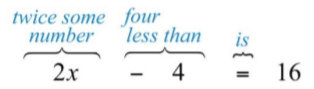
Four less than twice some number is \(16\).

First, choose a variable for the unknown number and identify the key words and phrases. Let \(x\) represent the unknown indicated by “some number.”

Figure \(\PageIndex{1}\)

Remember that subtraction is not commutative. For this reason, take care when setting up differences. In this example, \(4−2x=16\) is an incorrect translation.

\(2x−4=16\)

It is important to first identify the variable— let x represent… —and state in words what the unknown quantity is. This step not only makes your work more readable but also forces you to think about what you are looking for. Usually, if you know what you are asked to find, then the task of finding it is achievable.

Example \(\PageIndex{2}\)

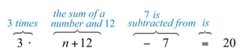
When \(7\) is subtracted from \(3\) times the sum of a number and \(12\), the result is \(20\).

Let \(n\) represent the unknown number.

Figure \(\PageIndex{2}\)

\(3(n+12)−7=20\)

To understand why parentheses are needed, study the structures of the following two sentences and their translations:

The key is to focus on the phrase “ 3 times the sum .” This prompts us to group the sum within parentheses and then multiply by 3. Once an application is translated into an algebraic equation, solve it using the techniques you have learned.

Guidelines for Setting Up and Solving Word Problems

• Step 1 : Read the problem several times, identify the key words and phrases, and organize the given information.
• Step 2 : Identify the variables by assigning a letter or expression to the unknown quantities.
• Step 3 : Translate and set up an algebraic equation that models the problem.
• Step 4 : Solve the resulting algebraic equation.
• Step 5 : Finally, answer the question in sentence form and make sure it makes sense (check it).

For now, set up all of your equations using only one variable. Avoid two variables by looking for a relationship between the unknowns.

Problems Involving Relationships between Real Numbers

We classify applications involving relationships between real numbers broadly as number problems. These problems can sometimes be solved using some creative arithmetic, guessing, and checking. Solving in this manner is not a good practice and should be avoided. Begin by working through the basic steps outlined in the general guidelines for solving word problems.

Example \(\PageIndex{3}\)

A larger integer is \(2\) less than \(3\) times a smaller integer. The sum of the two integers is \(18\). Find the integers.

Identify variables : Begin by assigning a variable to the smaller integer.

Let \(x\) represent the smaller integer.

Use the first sentence to identify the larger integer in terms of the variable \(x\): “A larger integer is 2 less than 3 times a smaller.”

Let \(3x-2\) represent the larger integer.

Set up an equation : Add the expressions that represent the two integers, and set the resulting expression equal to \(18\) as indicated in the second sentence: “The sum of the two integers is \(18\).”

\(x+(3x-2)=18\)

Solve : Solve the equation to obtain the smaller integer \(x\).

\(\begin{aligned} x+(3x-2)&=18 \\ x+3x-2&=18 \\ 4x-2&=18 \\ 4x-2\color{Cerulean}{+2}&=18\color{Cerulean}{+2} \\ 4x&=20 \\ \frac{4x}{\color{Cerulean}{4}}&=\frac{20}{\color{Cerulean}{4}} \\ x&=5 \end{aligned}\)

Back substitute : Use the expression \(3x−2\) to find the larger integer—this is called back substituting.

\(3x-2=3(\color{OliveGreen}{5}\color{black}{)-2=15-2=13}\)

Answer the question : The two integers are \(5\) and \(13\).

Check : \(5 + 13 = 18\). The answer makes sense.

Example \(\PageIndex{4}\)

The difference between two integers is \(2\). The larger integer is \(6\) less than twice the smaller. Find the integers.

Use the relationship between the two integers in the second sentence, “The larger integer is 6 less than twice the smaller ,” to identify the unknowns in terms of one variable.

Let \(2x-6\) represent the larger integer.

Since the difference is positive, subtract the smaller integer from the larger.

\((2x-6)-x=2\)

\(\begin{aligned} \color{OliveGreen}{2x}\color{black}{-6}\color{OliveGreen}{-x}&=2 \\ x-6&=2 \\ x-6\color{Cerulean}{+6}&=2\color{Cerulean}{+6} \\ x&=8 \end{aligned}\)

Use \(2x − 6\) to find the larger integer.

\(2x-6=2(\color{Cerulean}{8}\color{black}{)-6=16-6=10}\)

The two integers are \(8\) and \(10\). These integers clearly solve the problem.

It is worth mentioning again that you can often find solutions to simple problems by guessing and checking. This is so because the numbers are chosen to simplify the process of solving, so that the algebraic steps are not too tedious. You learn how to set up algebraic equations with easier problems, so that you can use these ideas to solve more difficult problems later.

Example \(\PageIndex{5}\)

• The sum of two consecutive even integers is \(46\). Find the integers.

The key phrase to focus on is “consecutive even integers.”

Let \(x\) represent the first even integer.

Let \(x+2\) represent the next even integer.

Add the even integers and set them equal to \(46\).

\(x+(x+2)=46\)

\(\begin{aligned}\color{OliveGreen}{x+x}\color{black}{+2}&=46\\2x+2&=46\\2x+2\color{Cerulean}{-2}&=46\color{Cerulean}{-2}\\2x&=44\\x&=22 \end{aligned}\)

Use \(x + 2\) to find the next even integer.

\(x+2=\color{Cerulean}{22}\color{black}{+2=24}\)

The consecutive even integers are \(22\) and \(24\).

It should be clear that consecutive even integers are separated by two units. However, it may not be so clear that odd integers are as well.

Figure \(\PageIndex{3}\)

Example \(\PageIndex{6}\)

The sum of two consecutive odd integers is \(36\). Find the integers.

The key phrase to focus on is “consecutive odd integers.”

Let \(x\) represent the first odd integer.

Let \(x+2\) represent the next odd integer.

Add the two odd integers and set the expression equal to \(36\).

\(x+(x+2)=36\)

\(\begin{aligned} \color{OliveGreen}{x+x}\color{black}{+2}&=36 \\ 2x+2&=36 \\ 2x+2\color{Cerulean}{-2}&=36\color{Cerulean}{-2} \\ 2x&=34 \\ \frac{2x}{\color{Cerulean}{2}}&=\frac{34}{\color{Cerulean}{2}} \\ x&=17 \end{aligned}\)

Use \(x + 2\) to find the next odd integer.

\(x+2=\color{OliveGreen}{17}\color{black}{+2=19}\)

The consecutive odd integers are \(17\) and \(19\).

The algebraic setup for even and odd integer problems is the same. A common mistake is to use \(x\) and \(x + 3\) when identifying the variables for consecutive odd integers. This is incorrect because adding 3 to an odd number yields an even number: for example, \(5 + 3 = 8\). An incorrect setup is very likely to lead to a decimal answer, which may be an indication that the problem was set up incorrectly.

Example \(\PageIndex{7}\)

The sum of three consecutive integers is \(24\). Find the integers.

Consecutive integers are separated by one unit.

Let \(x\) represent the first integer.

Let \(x+1\) represent the next integer.

Let \(x+2\) represent the third integer.

Add the integers and set the sum equal to \(24\).

\(x+(x+1)+(x+2)=24\)

\(\begin{aligned} \color{OliveGreen}{x+x}\color{black}{+1}\color{OliveGreen}{+x}\color{black}{+2}&=24\\ 3x+3&=24 \\ 3x+3\color{Cerulean}{-3}&=24\color{Cerulean}{-3} \\ 3x&=21 \\ x&=7 \end{aligned}\)

Back substitute to find the other two integers.

\(x+1=\color{OliveGreen}{7}\color{black}{+1=8}\)

\(x+2=\color{OliveGreen}{7}\color{black}{+2=9}\)

The three consecutive integers are \(7, 8\) and \(9\), where \(7 + 8 + 9 = 24\).

Exercise \(\PageIndex{1}\)

The sum of three consecutive odd integers is \(87\). Find the integers.

The integers are \(27, 29\), and \(31\).

Geometry Problems (Perimeter)

Recall that the perimeter of a polygon is the sum of the lengths of all the outside edges. In addition, it is helpful to review the following perimeter formulas \((π≈3.14159)\).

Keep in mind that you are looking for a relationship between the unknowns so that you can set up algebraic equations using only one variable. When working with geometry problems, it is often helpful to draw a picture.

Example \(\PageIndex{8}\)

A rectangle has a perimeter measuring \(64\) feet. The length is \(4\) feet more than \(3\) times the width. Find the dimensions of the rectangle.

The sentence “The length is 4 feet more than 3 times the width ” gives the relationship between the two variables.

Figure \(\PageIndex{4}\)

Let \(w\) represent the width of the rectangle.

Let \(3w+4\) represent the length.

The sentence “A rectangle has a perimeter measuring \(64\) feet” suggests an algebraic setup. Substitute \(64\) for the perimeter and the expression for the length into the appropriate formula as follows:

\(\begin{aligned} P&=\:\:\:\:\quad 2l + 2w \\ \color{Cerulean}{\downarrow}&\:\:\:\qquad\quad\color{Cerulean}{\downarrow} \\ \color{OliveGreen}{64}&=2(\color{OliveGreen}{3w+4}\color{black}{)+2w} \end{aligned}\)

Once you have set up an algebraic equation with one variable, solve for the width, \(w\).

\(\begin{aligned} 64&=\color{OliveGreen}{6w}\color{black}{+8+}\color{OliveGreen}{2w} \\ 64&=8w+8 \\ 64\color{Cerulean}{-8}&=8w+8\color{Cerulean}{-8} \\ 56&=8w \\ \frac{56}{\color{Cerulean}{8}}&=\frac{8w}{\color{Cerulean}{8}} \\ 7&=w \end{aligned}\)

Use \(3w + 4\) to find the length.

\(l=3w+4=3(\color{OliveGreen}{7}\color{black}{)+4=21+4=25}\)

The rectangle measures \(7\) feet by \(25\) feet. To check, add all of the sides:

\(P=7\text{ ft+}7\text{ ft+}25\text{ ft+}25\text{ ft}=64\text{ ft}\)

Example \(\PageIndex{9}\)

Two sides of a triangle are \(5\) and \(7\) inches longer than the third side. If the perimeter measures \(21\) inches, find the length of each side.

Figure \(\PageIndex{5}\)

The first sentence describes the relationships between the unknowns.

Let \(x\) represent the length of the third side.

Let \(x+5\) and \(x+7\) represent the lengths of the other two sides.

Substitute these expressions into the appropriate formula and use \(21\) for the perimeter \(P\).

\(\begin{aligned} P&=a+b+c \\ \color{OliveGreen}{21}&=\color{OliveGreen}{x}\color{black}{+}\color{OliveGreen}{(x+5)}\color{black}{+}\color{OliveGreen}{(x+7)} \end{aligned}\)

You now have an equation with one variable to solve.

\(\begin{aligned} 21&=x+x+5+x+7 \\ 21&=3x+12 \\ 21\color{Cerulean}{-12}&=3x+12\color{Cerulean}{-12} \\ 9&=3x\\ \frac{9}{\color{Cerulean}{3}}&=\frac{3x}{\color{Cerulean}{3}} \\ 3&=x \end{aligned}\)

Back substitute.

\(x+5=\color{OliveGreen}{3}\color{black}{+5=8}\)

\(x+5=\color{OliveGreen}{3}\color{black}{+7=10}\)

The three sides of the triangle measure \(3\) inches, \(8\) inches, and \(10\) inches. The check is left to the reader.

Exercise \(\PageIndex{2}\)

The length of a rectangle is \(1\) foot less than twice its width. If the perimeter is \(46\) feet, find the dimensions.

Width: \(8\) feet; length: \(15\) feet

Problems Involving Money and Percents

Whenever setting up an equation involving a percentage, we usually need to convert the percentage to a decimal or fraction. If the question asks for a percentage, then do not forget to convert your answer to a percent at the end. Also, when money is involved, be sure to round off to two decimal places.

Example \(\PageIndex{10}\)

If a pair of shoes costs $\(52.50\) including a \(7\frac{1}{4}\)% tax, what is the original cost of the item before taxes are added?

Begin by converting \(7\frac{1}{4}\)% to a decimal.

\(7\frac{1}{4}%=7.25%=0.0725\)

The amount of tax is this rate times the original cost of the item. The original cost of the item is what you are asked to find.

Let \(c\) represent the cost of the item \(\underline{\text{before taxes}}\) are added.

\(\color{Cerulean}{amount\:of\:tax\:=\:tax\:rate\:\cdot\:cost\:of\:item}\)

\(=0.0725\cdot c\)

\(\color{Cerulean}{total\:cost\:=\:cost\:of\:item\:+\:amount\:of\:tax}\)

\(52.50=c+0.0725c\)

Use this equation to solve for \(c\), the original cost of the item.

\(\begin{aligned} 52.50&=\color{OliveGreen}{1c+0.0725c} \\ 52.50&=1.0725c \\ \frac{52.50}{\color{Cerulean}{1.0725}}&=\frac{1.0725c}{\color{Cerulean}{1.0725}} \\ 48.95& \approx c \end{aligned}\)

The cost of the item before taxes is $\(48.95\). Check this by multiplying $\(48.95\) by \(0.0725\) to obtain the tax and add it to this cost.

Example \(\PageIndex{11}\)

Given a \(5\frac{1}{8}\)% annual interest rate, how long will it take $\(1,200\) to yield $\(307.50\) in simple interest?

Let \(t\) represent the time needed to earn $\(307.50\) at \(5.125\)%.

Organize the data needed to use the simple interest formula \(I=prt\).

Next, substitute all of the known quantities into the formula and then solve for the only unknown, \(t\).

\(\begin{aligned} I&=prt \\ \color{OliveGreen}{307.50}&=\color{OliveGreen}{1200}\color{black}{(}\color{OliveGreen}{0.05125}\color{black}{)t} \\ 307.50&=61.5t \\ \frac{307.50}{\color{Cerulean}{61.5}}&=\frac{61.5t}{\color{Cerulean}{61.5}} \\ 5&=t \end{aligned}\)

It takes \(5\) years for $\(1,200\) invested at \(5\frac{1}{8}\)% to earn $\(307.50\) in simple interest.

Example \(\PageIndex{12}\)

Mary invested her total savings of $\(3,400\) in two accounts. Her mutual fund account earned \(8\)% last year and her CD earned \(5\)%. If her total interest for the year was $\(245\), how much was in each account?

The relationship between the two unknowns is that they total $3,400. When a total is involved, a common technique used to avoid two variables is to represent the second unknown as the difference of the total and the first unknown.

Let \(x\) represent the amount invested in the mutual fund at \(8\)%\(=0.08\).

Let \(3,400-x\) represent the remaining amount invested in the CD at \(5\)%\(=0.05\).

The total interest is the sum of the interest earned from each account.

\(\color{Cerulean}{mutual\:fund\:interest\:+\:CD\:interest\:=\:total\:interest}\)

\(0.08x+0.05(3,400-x)=245\)

This equation models the problem with one variable. Solve for \(x\).

\(\begin{aligned} 0.08x+0.05(3,400-x)&=245 \\ \color{OliveGreen}{0.08x}\color{black}{+170}\color{OliveGreen}{-0.05x}&=245 \\ 0.03x+170\color{Cerulean}{-170} &=245\color{Cerulean}{-170} \\ 0.03x&=75 \\ \frac{0.03x}{\color{Cerulean}{0.03}}&=\frac{75}{\color{Cerulean}{0.03}} \\ x&=2,500 \end{aligned}\)

\(3,400-x=3,400-\color{OliveGreen}{2,500}\color{black}{=900}\)

Mary invested $\(2,500\) at \(8\)% in a mutual fund and $\(900\) at \(5\)% in a CD.

Example \(\PageIndex{13}\)

Joe has a handful of dimes and quarters that values $\(5.30\). He has one fewer than twice as many dimes than quarters. How many of each coin does he have?

Begin by identifying the variables.

Let \(q\) represent the number of quarters Joe is holding.

Let \(2q-1\) represent the number of dimes.

To determine the total value of a number of coins, multiply the number of coins by the value of each coin. For example, \(5\) quarters have a value $\(0.25 ⋅ 5 =\) $\(1.25\).

\(\color{Cerulean}{value\:in\:quarters\:+\:value\:in\:dimes\:=\:total\:value\:of\:coins}\)

\(0.25q+0.10(2q-1)=5.30\)

Solve for the number of quarters, \(q\).

\(\begin{aligned} 0.25q+0.10(2q-1)&=5.30 \\ \color{OliveGreen}{0.25q+0.20q}\color{black}{-0.10}&=5.30 \\ 0.45q-0.10&=5.30 \\ 0.45q-0.10\color{Cerulean}{+0.10}&=5.30\color{Cerulean}{+0.10} \\ 0.45q&=5.40 \\ \frac{0.45q}{\color{Cerulean}{0.45}}&=\frac{5.40}{\color{Cerulean}{0.45}} \\ q&=12 \end{aligned}\)

Back substitute into \(2q − 1\) to find the number of dimes.

\(2q-1=2(\color{OliveGreen}{12}\color{black}{)-1=24-1=23}\)

Joe has \(12\) quarters and \(23\) dimes. Check by multiplying $\(0.25 ⋅ 12 = \)$\(3.00\) and $\(0.10 ⋅ 23 = \)$\(2.30\). Then add to obtain the correct amount: $\(3.00 + \)$\(2.30 = \)$\(5.30\).

Exercise \(\PageIndex{3}\)

A total amount of $\(5,900\) is invested in two accounts. One account earns \(3.5\)% interest and another earns \(4.5\)%. If the interest for \(1\) year is $\(229.50\), then how much is invested in each account?

$\(3,600\) is invested at \(3.5\)% and $\(2,300\) at \(4.5\)%.

Uniform Motion Problems (Distance Problems)

Uniform motion refers to movement at a speed, or rate that does not change. We can determine the distance traveled by multiplying the average rate by the time traveled at that rate with the formula \(D=r⋅t\). Applications involving uniform motion usually have a lot of data, so it helps to first organize the data in a chart and then set up an algebraic equation that models the problem.

Example \(\PageIndex{14}\)

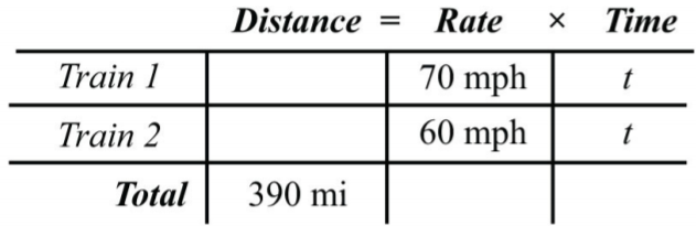
Two trains leave the station at the same time traveling in opposite directions. One travels at \(70\) miles per hour and the other at \(60\) miles per hour. How long does it take for the distance between them to reach \(390\) miles?

First, identify the unknown quantity and organize the data.

Let \(t\) represent the time it takes to separate \(390\) miles.

Figure \(\PageIndex{6}\)

The given information is filled in on the following chart. The time for each train is equal.

Figure \(\PageIndex{7}\)

To avoid introducing two more variables, use the formula \(D=r⋅t\) to fill in the unknown distances traveled by each train.

Distance traveled by train 1: \(D=r\cdot t=70\cdot t\)

Distance traveled by tain 2: \(D=r\cdot t=60\cdot t\)

We can now completely fill in the chart.

Figure \(\PageIndex{8}\)

The algebraic setup is defined by the distance column. The problem asks for the time it takes for the total distance to reach \(390\) miles.

Figure \(\PageIndex{9}\)

Solve for \(t\).

\(\begin{aligned} 70t+60t&=390 \\ 130t&=390 \\ \frac{130t}{\color{Cerulean}{130}}&=\frac{390}{\color{Cerulean}{130}} \\ t&=3 \end{aligned}\)

It takes \(3\) hours for the distance between the trains to reach \(390\) miles.

Example \(\PageIndex{15}\)

A train traveling nonstop to its destination is able to make the trip at an average speed of \(72\) miles per hour. On the return trip, the train makes several stops and is only able to average \(48\) miles per hour. If the return trip takes \(2\) hours longer than the initial trip to the destination, then what is the travel time each way?

Let \(t\) represent the time it takes to arrive at the destination.

Let \(t+2\) represent the time it takes for the return trip.

Figure \(\PageIndex{10}\)

The given information is filled in the following chart:

Figure \(\PageIndex{11}\)

Use the formula \(D=r⋅t\) to fill in the unknown distances.

Distance traveled on the destination: \(D=r\cdot t=72\cdot t\)

Distance traveled on the return trip: \(D=r\cdot t=48\cdot (t+2)\)

Use these expressions to complete the chart.

Figure \(\PageIndex{12}\)

The algebraic setup is again defined by the distance column. In this case, the distance to the destination and back is the same, and the equation is

\(72t=48(t+2)\)

\(\begin{aligned} 72t&=48(t+2) \\ 722&=48t+96 \\ 72t-48t&=48t+96-48t \\ 24t&=96 \\ \frac{24t}{24}&=\frac{96}{24} \\ t&=4 \end{aligned}\)

The return trip takes \(t+2=4+2=6\) hours.

It takes \(4\) hours to arrive at the destination and \(6\) hours to return.

Exercise \(\PageIndex{4}\)

Mary departs for school on a bicycle at an average rate of \(6\) miles per hour. Her sister Kate, running late, leaves \(15\) minutes later and cycles at twice that speed. How long will it take Kate to catch up to Mary? Be careful! Pay attention to the units given in the problem.

It takes \(15\) minutes for Kate to catch up.

Key Takeaways

• Simplify the process of solving real-world problems by creating mathematical models that describe the relationship between unknowns. Use algebra to solve the resulting equations.
• Guessing and checking for solutions is a poor practice. This technique might sometimes produce correct answers, but is unreliable, especially when problems become more complex.
• Read the problem several times and search for the key words and phrases. Identify the unknowns and assign variables or expressions to the unknown quantities. Look for relationships that allow you to use only one variable. Set up a mathematical model for the situation and use algebra to solve the equation. Check to see if the solution makes sense and present the solution in sentence form.
• Do not avoid word problems: solving them can be fun and rewarding. With lots of practice you will find that they really are not so bad after all. Modeling and solving applications is one of the major reasons to study algebra.
• Do not feel discouraged when the first attempt to solve a word problem does not work. This is part of the process. Try something different and learn from incorrect attempts.

Exercise \(\PageIndex{5}\) Translate

Translate the following into algebraic equations.

• The sum of a number and \(6\) is \(37\).
• When \(12\) is subtracted from twice some number the result is \(6\).
• Fourteen less than \(5\) times a number is \(1\).
• Twice some number is subtracted from \(30\) and the result is \(50\).
• Five times the sum of \(6\) and some number is \(20\).
• The sum of \(5\) times some number and \(6\) is \(20\).
• When the sum of a number and \(3\) is subtracted from \(10\) the result is \(5\).
• The sum of three times a number and five times that same number is \(24\).
• Ten is subtracted from twice some number and the result is the sum of the number and \(2\).
• Six less than some number is ten times the sum of that number and \(5\).

1. \(x+6=37\)

3. \(5x−14=1\)

5. \(5(x+6)=20\)

7. \(10−(x+3)=5\)

9. \(2x−10=x+2\)

Exercise \(\PageIndex{6}\) Number Problems

Set up an algebraic equation and then solve.

• A larger integer is \(1\) more than twice another integer. If the sum of the integers is \(25\), find the integers.
• If a larger integer is \(2\) more than \(4\) times another integer and their difference is \(32\), find the integers.
• One integer is \(30\) more than another integer. If the difference between the larger and twice the smaller is \(8\), find the integers.
• The quotient of some number and \(4\) is \(22\). Find the number.
• Eight times a number is decreased by three times the same number, giving a difference of \(20\). What is the number?
• One integer is two units less than another. If their sum is \(−22\), find the two integers.
• The sum of two consecutive integers is \(139\). Find the integers.
• The sum of three consecutive integers is \(63\). Find the integers.
• The sum of three consecutive integers is \(279\). Find the integers.
• The difference of twice the smaller of two consecutive integers and the larger is \(39\). Find the integers.
• If the smaller of two consecutive integers is subtracted from two times the larger, then the result is \(17\). Find the integers.
• The sum of two consecutive even integers is \(238\). Find the integers.
• The sum of three consecutive even integers is \(96\). Find the integers.
• If the smaller of two consecutive even integers is subtracted from \(3\) times the larger the result is \(42\). Find the integers.
• The sum of three consecutive even integers is \(90\). Find the integers.
• The sum of two consecutive odd integers is \(68\). Find the integers.
• The sum of two consecutive odd integers is \(180\). Find the integers.
• The sum of three consecutive odd integers is \(57\). Find the integers.
• If the smaller of two consecutive odd integers is subtracted from twice the larger the result is \(23\). Find the integers.
• Twice the sum of two consecutive odd integers is \(32\). Find the integers.
• The difference between twice the larger of two consecutive odd integers and the smaller is \(59\). Find the integers.

1. \(8, 17\)

3. \(22, 52\)

7. \(69, 70\)

9. \(92, 93, 94\)

11. \(15, 16\)

13. \(118, 120\)

15. \(18, 20\)

17. \(33, 35\)

19. \(17, 19, 21\)

21. \(7, 9\)

Exercise \(\PageIndex{7}\) Geometry Problems

• If the perimeter of a square is \(48\) inches, then find the length of each side.
• The length of a rectangle is \(2\) inches longer than its width. If the perimeter is \(36\) inches, find the length and width.
• The length of a rectangle is \(2\) feet less than twice its width. If the perimeter is \(26\) feet, find the length and width.
• The width of a rectangle is \(2\) centimeters less than one-half its length. If the perimeter is \(56\) centimeters, find the length and width.
• The length of a rectangle is \(3\) feet less than twice its width. If the perimeter is \(54\) feet, find the dimensions of the rectangle.
• If the length of a rectangle is twice as long as the width and its perimeter measures \(72\) inches, find the dimensions of the rectangle.
• The perimeter of an equilateral triangle measures \(63\) centimeters. Find the length of each side.
• An isosceles triangle whose base is one-half as long as the other two equal sides has a perimeter of \(25\) centimeters. Find the length of each side.
• Each of the two equal legs of an isosceles triangle are twice the length of the base. If the perimeter is \(105\) centimeters, then how long is each leg?
• A triangle has sides whose measures are consecutive even integers. If the perimeter is \(42\) inches, find the measure of each side.
• A triangle has sides whose measures are consecutive odd integers. If the perimeter is \(21\) inches, find the measure of each side.
• A triangle has sides whose measures are consecutive integers. If the perimeter is \(102\) inches, then find the measure of each side.
• The circumference of a circle measures \(50π\) units. Find the radius.
• The circumference of a circle measures \(10π\) units. Find the radius.
• The circumference of a circle measures \(100\) centimeters. Determine the radius to the nearest tenth.
• The circumference of a circle measures \(20\) centimeters. Find the diameter rounded off to the nearest hundredth.
• The diameter of a circle measures \(5\) inches. Determine the circumference to the nearest tenth.
• The diameter of a circle is \(13\) feet. Calculate the exact value of the circumference.

1. \(12\) inches

3. Width: \(5\) feet; length: \(8\) feet

5. Width: \(10\) feet; length: \(17\) feet

7. \(21\) centimeters

9. \(21\) centimeters, \(42\) centimeters, \(42\) centimeters

11. \(5\) inches, \(7\) inches, \(9\) inches

13. \(25\) units

15. \(15.9\) centimeters

17. \(15.7\) inches

Exercise \(\PageIndex{8}\) Percent and Money Problems

• Calculate the simple interest earned on a \(2\)-year investment of $\(1,550\) at a \(8\frac{3}{4}\)% annual interest rate.
• Calculate the simple interest earned on a \(1\)-year investment of $\(500\) at a \(6\)% annual interest rate.
• For how many years must $\(10,000\) be invested at an \(8\frac{1}{2}\)% annual interest rate to yield $\(4,250\) in simple interest?
• For how many years must $\(1,000\) be invested at a \(7.75\)% annual interest rate to yield $\(503.75\) in simple interest?
• At what annual interest rate must $\(2,500\) be invested for \(3\) years in order to yield $\(412.50\) in simple interest?
• At what annual interest rate must $\(500\) be invested for \(2\) years in order to yield $\(93.50\) in simple interest?
• If the simple interest earned for \(1\) year was $\(47.25\) and the annual rate was \(6.3\)%, what was the principal?
• If the simple interest earned for \(2\) years was $\(369.60\) and the annual rate was \(5\frac{1}{4}\)%, what was the principal?
• Joe invested last year’s $\(2,500\) tax return in two different accounts. He put most of the money in a money market account earning \(5\)% simple interest. He invested the rest in a CD earning \(8\)% simple interest. How much did he put in each account if the total interest for the year was $\(138.50\)?
• James invested $\(1,600\) in two accounts. One account earns \(4.25\)% simple interest and the other earns \(8.5\)%. If the interest after \(1\) year was $\(85\), how much did he invest in each account?
• Jane has her $\(5,400\) savings invested in two accounts. She has part of it in a CD at \(3\)% annual interest and the rest in a savings account that earns \(2\)% annual interest. If the simple interest earned from both accounts is $\(140\) for the year, then how much does she have in each account?
• Marty put last year’s bonus of $\(2,400\) into two accounts. He invested part in a CD with \(2.5\)% annual interest and the rest in a money market fund with \(1.3\)% annual interest. His total interest for the year was $\(42.00\). How much did he invest in each account?
• Alice puts money into two accounts, one with \(2\)% annual interest and another with \(3\)% annual interest. She invests \(3\) times as much in the higher yielding account as she does in the lower yielding account. If her total interest for the year is $\(27.50\), how much did she invest in each account?
• Jim invested an inheritance in two separate banks. One bank offered \(5.5\)% annual interest rate and the other \(6\frac{1}{4}\)%. He invested twice as much in the higher yielding bank account than he did in the other. If his total simple interest for \(1\) year was $\(4,860\), then what was the amount of his inheritance?
• If an item is advertised to cost $\(29.99\) plus \(9.25\)% tax, what is the total cost?
• If an item is advertised to cost $\(32.98\) plus \(8\frac{3}{4}\)% tax, what is the total cost?
• An item, including an \(8.75\)% tax, cost $\(46.49\). What is the original pretax cost of the item?
• An item, including a \(5.48\)% tax, cost $\(17.82\). What is the original pretax cost of the item?
• If a meal costs $\(32.75\), what is the total after adding a \(15\)% tip?
• How much is a \(15\)% tip on a restaurant bill that totals $\(33.33\)?
• Ray has a handful of dimes and nickels valuing $\(3.05\). He has \(5\) more dimes than he does nickels. How many of each coin does he have?
• Jill has \(3\) fewer half-dollars than she has quarters. The value of all \(27\) of her coins adds to $\(9.75\). How many of each coin does Jill have?
• Cathy has to deposit $\(410\) worth of five- and ten-dollar bills. She has \(1\) fewer than three times as many tens as she does five-dollar bills. How many of each bill does she have to deposit?
• Billy has a pile of quarters, dimes, and nickels that values $\(3.75\). He has \(3\) more dimes than quarters and \(5\) more nickels than quarters. How many of each coin does Billy have?
• Mary has a jar with one-dollar bills, half-dollar coins, and quarters valuing $\(14.00\). She has twice as many quarters than she does half-dollar coins and the same amount of half-dollar coins as one-dollar bills. How many of each does she have?
• Chad has a bill-fold of one-, five-, and ten-dollar bills totaling $\(118\). He has \(2\) more than \(3\) times as many ones as he does five-dollar bills and \(1\) fewer ten- than five-dollar bills. How many of each bill does Chad have?

1. $\(271.25\)

3. \(5\) years

5. \(5.5\)%

7. $\(750.00\)

9. Joe invested $\(2,050\) in the money market account and $\(450\) in the CD.

11. Jane has $\(3,200\) in the CD and $\(2,200\) in savings.

13. Alice invested $\(250\) at \(2\)% and $\(750\) at a \(3\)%.

15. $\(32.76\)

17. $\(42.75\)

19. $\(37.66\)

21. He has \(17\) nickels and \(22\) dimes.

23. Cathy has \(12\) fives and \(35\) ten-dollar bills.

25. Mary has \(7\) one-dollar bills, \(7\) half-dollar coins, and \(14\) quarters.

Exercise \(\PageIndex{9}\) Uniform Motion (Distance Problems)

Set up an algebraic equation then solve.

• Two cars leave a location traveling in opposite directions. If one car averages \(55\) miles per hour and the other averages \(65\) miles per hour, then how long will it take for them to separate a distance of \(300\) miles?
• Two planes leave the airport at the same time traveling in opposite directions. The average speeds for the planes are \(450\) miles per hour and \(395\) miles per hour. How long will it take the planes to be a distance of \(1,478.75\) miles apart?
• Bill and Ted are racing across the country. Bill leaves \(1\) hour earlier than Ted and travels at an average rate of \(60\) miles per hour. If Ted intends to catch up at a rate of \(70\) miles per hour, then how long will it take?
• Two brothers leave from the same location, one in a car and the other on a bicycle, to meet up at their grandmother’s house for dinner. If one brother averages \(30\) miles per hour in the car and the other averages \(12\) miles per hour on the bicycle, then it takes the brother on the bicycle \(1\) hour less than \(3\) times as long as the other in the car. How long does it take each of them to make the trip?
• A commercial airline pilot flew at an average speed of \(350\) miles per hour before being informed that his destination airfield may be closed due to poor weather conditions. In an attempt to arrive before the storm, he increased his speed \(400\) miles per hour and flew for another \(3\) hours. If the total distance flown was \(2,950\) miles, then how long did the trip take?
• Two brothers drove the \(2,793\) miles from Los Angeles to New York. One of the brothers, driving during the day, was able to average \(70\) miles per hour, and the other, driving at night, was able to average \(53\) miles per hour. If the brother driving at night drove \(3\) hours less than the brother driving in the day, then how many hours did they each drive?
• Joe and Ellen live \(21\) miles apart. Departing at the same time, they cycle toward each other. If Joe averages \(8\) miles per hour and Ellen averages \(6\) miles per hour, how long will it take them to meet?
• If it takes \(6\) minutes to drive to the automobile repair shop at an average speed of \(30\) miles per hour, then how long will it take to walk back at an average rate of \(4\) miles per hour?
• Jaime and Alex leave the same location and travel in opposite directions. Traffic conditions enabled Alex to average \(14\) miles per hour faster than Jaime. After \(1\frac{1}{2}\) hours they are \(159\) miles apart. Find the speed at which each was able to travel.
• Jane and Holly live \(51\) miles apart and leave at the same time traveling toward each other to meet for lunch. Jane traveled on the freeway at twice the average speed as Holly. They were able to meet in a half hour. At what rate did each travel?

1. \(2.5\) hours

3. \(6\) hours

5. \(8\) hours

7. \(1\frac{1}{2}\) hours

9. Jaime: \(46\) miles per hour; Alex: \(60\) miles per hour

Exercise \(\PageIndex{10}\) Discussion Board Topics

• Discuss ideas for calculating taxes and tips mentally.
• Research historical methods for representing unknowns.
• Research and compare simple interest and compound interest. What is the difference?
• Discuss why algebra is a required subject.
• Research ways to show that a repeating decimal is rational. Share your findings on the discussion board.

1. Answers may vary

3. Answers may vary

5. Answers may vary

Emery Evans

receive 15% off

Finished Papers

Frequently Asked Questions