4.1 Solve Systems of Linear Equations with Two Variables
Learning objectives.
By the end of this section, you will be able to:
- Determine whether an ordered pair is a solution of a system of equations
- Solve a system of linear equations by graphing
- Solve a system of equations by substitution
- Solve a system of equations by elimination
- Choose the most convenient method to solve a system of linear equations

Be Prepared 4.1
Before you get started, take this readiness quiz.
For the equation y = 2 3 x − 4 , y = 2 3 x − 4 , ⓐ Is ( 6 , 0 ) ( 6 , 0 ) a solution? ⓑ Is ( −3 , −2 ) ( −3 , −2 ) a solution? If you missed this problem, review Example 3.2 .
Be Prepared 4.2
Find the slope and y -intercept of the line 3 x − y = 12 . 3 x − y = 12 . If you missed this problem, review Example 3.16 .
Be Prepared 4.3
Find the x- and y -intercepts of the line 2 x − 3 y = 12 . 2 x − 3 y = 12 . If you missed this problem, review Example 3.8 .
Determine Whether an Ordered Pair is a Solution of a System of Equations
In Solving Linear Equations , we learned how to solve linear equations with one variable. Now we will work with two or more linear equations grouped together, which is known as a system of linear equations .
System of Linear Equations
When two or more linear equations are grouped together, they form a system of linear equations .
In this section, we will focus our work on systems of two linear equations in two unknowns. We will solve larger systems of equations later in this chapter.
An example of a system of two linear equations is shown below. We use a brace to show the two equations are grouped together to form a system of equations.
A linear equation in two variables, such as 2 x + y = 7 , 2 x + y = 7 , has an infinite number of solutions. Its graph is a line. Remember, every point on the line is a solution to the equation and every solution to the equation is a point on the line.
To solve a system of two linear equations, we want to find the values of the variables that are solutions to both equations. In other words, we are looking for the ordered pairs ( x , y ) ( x , y ) that make both equations true. These are called the solutions of a system of equations .
Solutions of a System of Equations
The solutions of a system of equations are the values of the variables that make all the equations true. A solution of a system of two linear equations is represented by an ordered pair ( x , y ) . ( x , y ) .
To determine if an ordered pair is a solution to a system of two equations, we substitute the values of the variables into each equation. If the ordered pair makes both equations true, it is a solution to the system.
Example 4.1
Determine whether the ordered pair is a solution to the system { x − y = −1 2 x − y = −5 . { x − y = −1 2 x − y = −5 .
ⓐ ( −2 , −1 ) ( −2 , −1 ) ⓑ ( −4 , −3 ) ( −4 , −3 )
Determine whether the ordered pair is a solution to the system { 3 x + y = 0 x + 2 y = −5 . { 3 x + y = 0 x + 2 y = −5 .
ⓐ ( 1 , −3 ) ( 1 , −3 ) ⓑ ( 0 , 0 ) ( 0 , 0 )
Determine whether the ordered pair is a solution to the system { x − 3 y = −8 − 3 x − y = 4 . { x − 3 y = −8 − 3 x − y = 4 .
ⓐ ( 2 , −2 ) ( 2 , −2 ) ⓑ ( −2 , 2 ) ( −2 , 2 )
Solve a System of Linear Equations by Graphing
In this section, we will use three methods to solve a system of linear equations. The first method we’ll use is graphing.
The graph of a linear equation is a line. Each point on the line is a solution to the equation. For a system of two equations, we will graph two lines. Then we can see all the points that are solutions to each equation. And, by finding what the lines have in common, we’ll find the solution to the system.
Most linear equations in one variable have one solution, but we saw that some equations, called contradictions, have no solutions and for other equations, called identities, all numbers are solutions.
Similarly, when we solve a system of two linear equations represented by a graph of two lines in the same plane, there are three possible cases, as shown.
Each time we demonstrate a new method, we will use it on the same system of linear equations. At the end of the section you’ll decide which method was the most convenient way to solve this system.
Example 4.2
How to solve a system of equations by graphing.
Solve the system by graphing { 2 x + y = 7 x − 2 y = 6 . { 2 x + y = 7 x − 2 y = 6 .
Solve the system by graphing: { x − 3 y = −3 x + y = 5 . { x − 3 y = −3 x + y = 5 .
Solve the system by graphing: { − x + y = 1 3 x + 2 y = 12 . { − x + y = 1 3 x + 2 y = 12 .
The steps to use to solve a system of linear equations by graphing are shown here.
Solve a system of linear equations by graphing.
- Step 1. Graph the first equation.
- Step 2. Graph the second equation on the same rectangular coordinate system.
- Step 3. Determine whether the lines intersect, are parallel, or are the same line.
- If the lines intersect, identify the point of intersection. This is the solution to the system.
- If the lines are parallel, the system has no solution.
- If the lines are the same, the system has an infinite number of solutions.
- Step 5. Check the solution in both equations.
In the next example, we’ll first re-write the equations into slope–intercept form as this will make it easy for us to quickly graph the lines.
Example 4.3
Solve the system by graphing: { 3 x + y = − 1 2 x + y = 0 . { 3 x + y = − 1 2 x + y = 0 .
We’ll solve both of these equations for y y so that we can easily graph them using their slopes and y -intercepts.
| Solve the first equation for . | |
| Find the slope and -intercept. | |
| Solve the second equation for . | |
| Find the slope and -intercept. | |
| Graph the lines. | |
| Determine the point of intersection. | The lines intersect at |
| Check the solution in both equations. | |
| The solution is |
Solve the system by graphing: { − x + y = 1 2 x + y = 10 . { − x + y = 1 2 x + y = 10 .
Solve the system by graphing: { 2 x + y = 6 x + y = 1 . { 2 x + y = 6 x + y = 1 .
In all the systems of linear equations so far, the lines intersected and the solution was one point. In the next two examples, we’ll look at a system of equations that has no solution and at a system of equations that has an infinite number of solutions.
Example 4.4
Solve the system by graphing: { y = 1 2 x − 3 x − 2 y = 4 . { y = 1 2 x − 3 x − 2 y = 4 .
| To graph the first equation, we will use its slope and -intercept. | |
| To graph the second equation, we will use the intercepts. | |
| Graph the lines. | |
| Determine the points of intersection. | The lines are parallel. Since no point is on both lines, there is no ordered pair that makes both equations true. There is no solution to this system. |
Solve the system by graphing: { y = − 1 4 x + 2 x + 4 y = − 8 . { y = − 1 4 x + 2 x + 4 y = − 8 .
Solve the system by graphing: { y = 3 x − 1 6 x − 2 y = 6 . { y = 3 x − 1 6 x − 2 y = 6 .
Sometimes the equations in a system represent the same line. Since every point on the line makes both equations true, there are infinitely many ordered pairs that make both equations true. There are infinitely many solutions to the system.
Example 4.5
Solve the system by graphing: { y = 2 x − 3 − 6 x + 3 y = − 9 . { y = 2 x − 3 − 6 x + 3 y = − 9 .
| Find the slope and -intercept of the first equation. | |
| Find the intercepts of the second equation. | |
| Graph the lines. | |
| The lines are the same! Since every point on the line makes both equations true, there are infinitely many ordered pairs that make both equations true. There are infinitely many solutions to this system. |
If you write the second equation in slope-intercept form, you may recognize that the equations have the same slope and same y -intercept.
Solve the system by graphing: { y = − 3 x − 6 6 x + 2 y = − 12 . { y = − 3 x − 6 6 x + 2 y = − 12 .
Try It 4.10
Solve the system by graphing: { y = 1 2 x − 4 2 x − 4 y = 16 . { y = 1 2 x − 4 2 x − 4 y = 16 .
When we graphed the second line in the last example, we drew it right over the first line. We say the two lines are coincident . Coincident lines have the same slope and same y- intercept.
Coincident Lines
Coincident lines have the same slope and same y- intercept.
The systems of equations in Example 4.2 and Example 4.3 each had two intersecting lines. Each system had one solution.
In Example 4.5 , the equations gave coincident lines, and so the system had infinitely many solutions.
The systems in those three examples had at least one solution. A system of equations that has at least one solution is called a consistent system.
A system with parallel lines, like Example 4.4 , has no solution. We call a system of equations like this inconsistent. It has no solution.
Consistent and Inconsistent Systems
A consistent system of equations is a system of equations with at least one solution.
An inconsistent system of equations is a system of equations with no solution.
We also categorize the equations in a system of equations by calling the equations independent or dependent . If two equations are independent, they each have their own set of solutions. Intersecting lines and parallel lines are independent.
If two equations are dependent, all the solutions of one equation are also solutions of the other equation. When we graph two dependent equations, we get coincident lines.
Let’s sum this up by looking at the graphs of the three types of systems. See below and Table 4.1 .
| Lines | Intersecting | Parallel | Coincident |
|---|---|---|---|
| 1 point | No solution | Infinitely many | |
| Consistent | Inconsistent | Consistent | |
| Independent | Independent | Dependent |
Example 4.6
Without graphing, determine the number of solutions and then classify the system of equations.
ⓐ { y = 3 x − 1 6 x − 2 y = 12 { y = 3 x − 1 6 x − 2 y = 12 ⓑ { 2 x + y = − 3 x − 5 y = 5 { 2 x + y = − 3 x − 5 y = 5
ⓐ We will compare the slopes and intercepts of the two lines.
| The first equation is already in slope-intercept form. | |
| Write the second equation in slope-intercept form. | |
| Find the slope and intercept of each line. | |
| Since the slopes are the same and -intercepts are different, the lines are parallel. |
A system of equations whose graphs are parallel lines has no solution and is inconsistent and independent.
ⓑ We will compare the slope and intercepts of the two lines.
| Write both equations in slope–intercept form. | |
| Find the slope and intercept of each line. | |
| Since the slopes are different, the lines intersect. |
A system of equations whose graphs are intersect has 1 solution and is consistent and independent.
Try It 4.11
ⓐ { y = −2 x − 4 4 x + 2 y = 9 { y = −2 x − 4 4 x + 2 y = 9 ⓑ { 3 x + 2 y = 2 2 x + y = 1 { 3 x + 2 y = 2 2 x + y = 1
Try It 4.12
ⓐ { y = 1 3 x − 5 x − 3 y = 6 { y = 1 3 x − 5 x − 3 y = 6 ⓑ { x + 4 y = 12 − x + y = 3 { x + 4 y = 12 − x + y = 3
Solving systems of linear equations by graphing is a good way to visualize the types of solutions that may result. However, there are many cases where solving a system by graphing is inconvenient or imprecise. If the graphs extend beyond the small grid with x and y both between −10 −10 and 10, graphing the lines may be cumbersome. And if the solutions to the system are not integers, it can be hard to read their values precisely from a graph.
Solve a System of Equations by Substitution
We will now solve systems of linear equations by the substitution method.
We will use the same system we used first for graphing.
We will first solve one of the equations for either x or y . We can choose either equation and solve for either variable—but we’ll try to make a choice that will keep the work easy.
Then we substitute that expression into the other equation. The result is an equation with just one variable—and we know how to solve those!
After we find the value of one variable, we will substitute that value into one of the original equations and solve for the other variable. Finally, we check our solution and make sure it makes both equations true.
Example 4.7
How to solve a system of equations by substitution.
Solve the system by substitution: { 2 x + y = 7 x − 2 y = 6 . { 2 x + y = 7 x − 2 y = 6 .
Try It 4.13
Solve the system by substitution: { − 2 x + y = −11 x + 3 y = 9 . { − 2 x + y = −11 x + 3 y = 9 .
Try It 4.14
Solve the system by substitution: { 2 x + y = −1 4 x + 3 y = 3 . { 2 x + y = −1 4 x + 3 y = 3 .
Solve a system of equations by substitution.
- Step 1. Solve one of the equations for either variable.
- Step 2. Substitute the expression from Step 1 into the other equation.
- Step 3. Solve the resulting equation.
- Step 4. Substitute the solution in Step 3 into either of the original equations to find the other variable.
- Step 5. Write the solution as an ordered pair.
- Step 6. Check that the ordered pair is a solution to both original equations.
Be very careful with the signs in the next example.
Example 4.8
Solve the system by substitution: { 4 x + 2 y = 4 6 x − y = 8 . { 4 x + 2 y = 4 6 x − y = 8 .
We need to solve one equation for one variable. We will solve the first equation for y .
| Solve the first equation for . Substitute for in the second equation. | |
| Replace the with | |
| Solve the equation for . | |
| Substitute into to find . | |
| The ordered pair is | |
| Check the ordered pair in both equations. | |
| The solution is |
Try It 4.15
Solve the system by substitution: { x − 4 y = −4 − 3 x + 4 y = 0 . { x − 4 y = −4 − 3 x + 4 y = 0 .
Try It 4.16
Solve the system by substitution: { 4 x − y = 0 2 x − 3 y = 5 . { 4 x − y = 0 2 x − 3 y = 5 .
Solve a System of Equations by Elimination
We have solved systems of linear equations by graphing and by substitution. Graphing works well when the variable coefficients are small and the solution has integer values. Substitution works well when we can easily solve one equation for one of the variables and not have too many fractions in the resulting expression.
The third method of solving systems of linear equations is called the Elimination Method. When we solved a system by substitution, we started with two equations and two variables and reduced it to one equation with one variable. This is what we’ll do with the elimination method, too, but we’ll have a different way to get there.
The Elimination Method is based on the Addition Property of Equality. The Addition Property of Equality says that when you add the same quantity to both sides of an equation, you still have equality. We will extend the Addition Property of Equality to say that when you add equal quantities to both sides of an equation, the results are equal.
For any expressions a, b, c, and d .
To solve a system of equations by elimination, we start with both equations in standard form. Then we decide which variable will be easiest to eliminate. How do we decide? We want to have the coefficients of one variable be opposites, so that we can add the equations together and eliminate that variable.
Notice how that works when we add these two equations together:
The y ’s add to zero and we have one equation with one variable.
Let’s try another one:
This time we don’t see a variable that can be immediately eliminated if we add the equations.
But if we multiply the first equation by −2 , −2 , we will make the coefficients of x opposites. We must multiply every term on both sides of the equation by −2 . −2 .
Then rewrite the system of equations.
Now we see that the coefficients of the x terms are opposites, so x will be eliminated when we add these two equations.
Once we get an equation with just one variable, we solve it. Then we substitute that value into one of the original equations to solve for the remaining variable. And, as always, we check our answer to make sure it is a solution to both of the original equations.
Now we’ll see how to use elimination to solve the same system of equations we solved by graphing and by substitution.
Example 4.9
How to solve a system of equations by elimination.
Solve the system by elimination: { 2 x + y = 7 x − 2 y = 6 . { 2 x + y = 7 x − 2 y = 6 .
Try It 4.17
Solve the system by elimination: { 3 x + y = 5 2 x − 3 y = 7 . { 3 x + y = 5 2 x − 3 y = 7 .
Try It 4.18
Solve the system by elimination: { 4 x + y = − 5 − 2 x − 2 y = − 2 . { 4 x + y = − 5 − 2 x − 2 y = − 2 .
The steps are listed here for easy reference.
Solve a system of equations by elimination.
- Step 1. Write both equations in standard form. If any coefficients are fractions, clear them.
- Decide which variable you will eliminate.
- Multiply one or both equations so that the coefficients of that variable are opposites.
- Step 3. Add the equations resulting from Step 2 to eliminate one variable.
- Step 4. Solve for the remaining variable.
- Step 5. Substitute the solution from Step 4 into one of the original equations. Then solve for the other variable.
- Step 6. Write the solution as an ordered pair.
- Step 7. Check that the ordered pair is a solution to both original equations.
Now we’ll do an example where we need to multiply both equations by constants in order to make the coefficients of one variable opposites.
Example 4.10
Solve the system by elimination: { 4 x − 3 y = 9 7 x + 2 y = −6 . { 4 x − 3 y = 9 7 x + 2 y = −6 .
In this example, we cannot multiply just one equation by any constant to get opposite coefficients. So we will strategically multiply both equations by different constants to get the opposites.
| Both equations are in standard form. To get opposite coefficients of , we will multiply the first equation by 2 and the second equation by 3. | |
| Simplify. | |
| Add the two equations to eliminate . | |
| Solve for . | |
| Substitute into one of the original equations. | |
| Solve for . | |
| Write the solution as an ordered pair. | The ordered pair is |
| Check that the ordered pair is a solution to original equations. | |
| The solution is |
Try It 4.19
Solve the system by elimination: { 3 x − 4 y = − 9 5 x + 3 y = 14 . { 3 x − 4 y = − 9 5 x + 3 y = 14 .
Try It 4.20
Solve each system by elimination: { 7 x + 8 y = 4 3 x − 5 y = 27 . { 7 x + 8 y = 4 3 x − 5 y = 27 .
When the system of equations contains fractions, we will first clear the fractions by multiplying each equation by the LCD of all the fractions in the equation.
Example 4.11
Solve the system by elimination: { x + 1 2 y = 6 3 2 x + 2 3 y = 17 2 . { x + 1 2 y = 6 3 2 x + 2 3 y = 17 2 .
In this example, both equations have fractions. Our first step will be to multiply each equation by the LCD of all the fractions in the equation to clear the fractions.
| To clear the fractions, multiply each equation by its LCD. | |
| Simplify. | |
| Now we are ready to eliminate one of the variables. Notice that both equations are in standard form. | |
| We can eliminate by multiplying the top equation by | |
| Simplify and add. Substitute into one of the original equations. | |
| Solve for . | |
| Write the solution as an ordered pair. | The ordered pair is |
| Check that the ordered pair is a solution to both original equations. | |
| The solution is |
Try It 4.21
Solve each system by elimination: { 1 3 x − 1 2 y = 1 3 4 x − y = 5 2 . { 1 3 x − 1 2 y = 1 3 4 x − y = 5 2 .
Try It 4.22
Solve each system by elimination: { x + 3 5 y = − 1 5 − 1 2 x − 2 3 y = 5 6 . { x + 3 5 y = − 1 5 − 1 2 x − 2 3 y = 5 6 .
When we solved the system by graphing, we saw that not all systems of linear equations have a single ordered pair as a solution. When the two equations were really the same line, there were infinitely many solutions. We called that a consistent system. When the two equations described parallel lines, there was no solution. We called that an inconsistent system.
The same is true using substitution or elimination. If the equation at the end of substitution or elimination is a true statement, we have a consistent but dependent system and the system of equations has infinitely many solutions. If the equation at the end of substitution or elimination is a false statement, we have an inconsistent system and the system of equations has no solution.
Example 4.12
Solve the system by elimination: { 3 x + 4 y = 12 y = 3 − 3 4 x . { 3 x + 4 y = 12 y = 3 − 3 4 x .
| Write the second equation in standard form. | |
| Clear the fractions by multiplying the second equation by 4. | |
| Simplify. | |
| To eliminate a variable, we multiply the second equation by −1. Simplify and add. |
This is a true statement. The equations are consistent but dependent. Their graphs would be the same line. The system has infinitely many solutions.
After we cleared the fractions in the second equation, did you notice that the two equations were the same? That means we have coincident lines.
Try It 4.23
Solve the system by elimination: { 5 x − 3 y = 15 y = − 5 + 5 3 x . { 5 x − 3 y = 15 y = − 5 + 5 3 x .
Try It 4.24
Solve the system by elimination: { x + 2 y = 6 y = − 1 2 x + 3 . { x + 2 y = 6 y = − 1 2 x + 3 .
Choose the Most Convenient Method to Solve a System of Linear Equations
When you solve a system of linear equations in in an application, you will not be told which method to use. You will need to make that decision yourself. So you’ll want to choose the method that is easiest to do and minimizes your chance of making mistakes.
Example 4.13
For each system of linear equations, decide whether it would be more convenient to solve it by substitution or elimination. Explain your answer.
ⓐ { 3 x + 8 y = 40 7 x − 4 y = −32 { 3 x + 8 y = 40 7 x − 4 y = −32 ⓑ { 5 x + 6 y = 12 y = 2 3 x − 1 { 5 x + 6 y = 12 y = 2 3 x − 1
Since both equations are in standard form, using elimination will be most convenient.
Since one equation is already solved for y , using substitution will be most convenient.
Try It 4.25
For each system of linear equations decide whether it would be more convenient to solve it by substitution or elimination. Explain your answer.
ⓐ { 4 x − 5 y = −32 3 x + 2 y = −1 { 4 x − 5 y = −32 3 x + 2 y = −1 ⓑ { x = 2 y − 1 3 x − 5 y = −7 { x = 2 y − 1 3 x − 5 y = −7
Try It 4.26
ⓐ { y = 2 x − 1 3 x − 4 y = − 6 { y = 2 x − 1 3 x − 4 y = − 6 ⓑ { 6 x − 2 y = 12 3 x + 7 y = −13 { 6 x − 2 y = 12 3 x + 7 y = −13
Section 4.1 Exercises
Practice makes perfect.
In the following exercises, determine if the following points are solutions to the given system of equations.
{ 2 x − 6 y = 0 3 x − 4 y = 5 { 2 x − 6 y = 0 3 x − 4 y = 5
ⓐ ( 3 , 1 ) ( 3 , 1 ) ⓑ ( −3 , 4 ) ( −3 , 4 )
{ − 3 x + y = 8 − x + 2 y = −9 { − 3 x + y = 8 − x + 2 y = −9
ⓐ ( −5 , −7 ) ( −5 , −7 ) ⓑ ( −5 , 7 ) ( −5 , 7 )
{ x + y = 2 y = 3 4 x { x + y = 2 y = 3 4 x
ⓐ ( 8 7 , 6 7 ) ( 8 7 , 6 7 ) ⓑ ( 1 , 3 4 ) ( 1 , 3 4 )
{ 2 x + 3 y = 6 y = 2 3 x + 2 { 2 x + 3 y = 6 y = 2 3 x + 2 ⓐ ( −6 , 2 ) ( −6 , 2 ) ⓑ ( −3 , 4 ) ( −3 , 4 )
In the following exercises, solve the following systems of equations by graphing.
{ 3 x + y = −3 2 x + 3 y = 5 { 3 x + y = −3 2 x + 3 y = 5
{ − x + y = 2 2 x + y = −4 { − x + y = 2 2 x + y = −4
{ y = x + 2 y = −2 x + 2 { y = x + 2 y = −2 x + 2
{ y = x − 2 y = −3 x + 2 { y = x − 2 y = −3 x + 2
{ y = 3 2 x + 1 y = − 1 2 x + 5 { y = 3 2 x + 1 y = − 1 2 x + 5
{ y = 2 3 x − 2 y = − 1 3 x − 5 { y = 2 3 x − 2 y = − 1 3 x − 5
{ x + y = −4 − x + 2 y = −2 { x + y = −4 − x + 2 y = −2
{ − x + 3 y = 3 x + 3 y = 3 { − x + 3 y = 3 x + 3 y = 3
{ − 2 x + 3 y = 3 x + 3 y = 12 { − 2 x + 3 y = 3 x + 3 y = 12
{ 2 x − y = 4 2 x + 3 y = 12 { 2 x − y = 4 2 x + 3 y = 12
{ x + 3 y = −6 y = − 4 3 x + 4 { x + 3 y = −6 y = − 4 3 x + 4
{ − x + 2 y = −6 y = − 1 2 x − 1 { − x + 2 y = −6 y = − 1 2 x − 1
{ − 2 x + 4 y = 4 y = 1 2 x { − 2 x + 4 y = 4 y = 1 2 x
{ 3 x + 5 y = 10 y = − 3 5 x + 1 { 3 x + 5 y = 10 y = − 3 5 x + 1
{ 4 x − 3 y = 8 8 x − 6 y = 14 { 4 x − 3 y = 8 8 x − 6 y = 14
{ x + 3 y = 4 − 2 x − 6 y = 3 { x + 3 y = 4 − 2 x − 6 y = 3
{ x = −3 y + 4 2 x + 6 y = 8 { x = −3 y + 4 2 x + 6 y = 8
{ 4 x = 3 y + 7 8 x − 6 y = 14 { 4 x = 3 y + 7 8 x − 6 y = 14
{ 2 x + y = 6 − 8 x − 4 y = −24 { 2 x + y = 6 − 8 x − 4 y = −24
{ 5 x + 2 y = 7 − 10 x − 4 y = −14 { 5 x + 2 y = 7 − 10 x − 4 y = −14
{ y = 2 3 x + 1 − 2 x + 3 y = 5 { y = 2 3 x + 1 − 2 x + 3 y = 5
{ y = 3 2 x + 1 2 x − 3 y = 7 { y = 3 2 x + 1 2 x − 3 y = 7
{ 5 x + 3 y = 4 2 x − 3 y = 5 { 5 x + 3 y = 4 2 x − 3 y = 5
{ y = − 1 2 x + 5 x + 2 y = 10 { y = − 1 2 x + 5 x + 2 y = 10
{ 5 x − 2 y = 10 y = 5 2 x − 5 { 5 x − 2 y = 10 y = 5 2 x − 5
In the following exercises, solve the systems of equations by substitution.
{ 2 x + y = −4 3 x − 2 y = −6 { 2 x + y = −4 3 x − 2 y = −6
{ 2 x + y = −2 3 x − y = 7 { 2 x + y = −2 3 x − y = 7
{ x − 2 y = −5 2 x − 3 y = −4 { x − 2 y = −5 2 x − 3 y = −4
{ x − 3 y = −9 2 x + 5 y = 4 { x − 3 y = −9 2 x + 5 y = 4
{ 5 x − 2 y = −6 y = 3 x + 3 { 5 x − 2 y = −6 y = 3 x + 3
{ − 2 x + 2 y = 6 y = −3 x + 1 { − 2 x + 2 y = 6 y = −3 x + 1
{ 2 x + 5 y = 1 y = 1 3 x − 2 { 2 x + 5 y = 1 y = 1 3 x − 2
{ 3 x + 4 y = 1 y = − 2 5 x + 2 { 3 x + 4 y = 1 y = − 2 5 x + 2
{ 2 x + y = 5 x − 2 y = −15 { 2 x + y = 5 x − 2 y = −15
{ 4 x + y = 10 x − 2 y = −20 { 4 x + y = 10 x − 2 y = −20
{ y = −2 x − 1 y = − 1 3 x + 4 { y = −2 x − 1 y = − 1 3 x + 4
{ y = x − 6 y = − 3 2 x + 4 { y = x − 6 y = − 3 2 x + 4
{ x = 2 y 4 x − 8 y = 0 { x = 2 y 4 x − 8 y = 0
{ 2 x − 16 y = 8 − x − 8 y = −4 { 2 x − 16 y = 8 − x − 8 y = −4
{ y = 7 8 x + 4 − 7 x + 8 y = 6 { y = 7 8 x + 4 − 7 x + 8 y = 6
{ y = − 2 3 x + 5 2 x + 3 y = 11 { y = − 2 3 x + 5 2 x + 3 y = 11
In the following exercises, solve the systems of equations by elimination.
{ 5 x + 2 y = 2 − 3 x − y = 0 { 5 x + 2 y = 2 − 3 x − y = 0
{ 6 x − 5 y = −1 2 x + y = 13 { 6 x − 5 y = −1 2 x + y = 13
{ 2 x − 5 y = 7 3 x − y = 17 { 2 x − 5 y = 7 3 x − y = 17
{ 5 x − 3 y = −1 2 x − y = 2 { 5 x − 3 y = −1 2 x − y = 2
{ 3 x − 5 y = −9 5 x + 2 y = 16 { 3 x − 5 y = −9 5 x + 2 y = 16
{ 4 x − 3 y = 3 2 x + 5 y = −31 { 4 x − 3 y = 3 2 x + 5 y = −31
{ 3 x + 8 y = −3 2 x + 5 y = −3 { 3 x + 8 y = −3 2 x + 5 y = −3
{ 11 x + 9 y = −5 7 x + 5 y = −1 { 11 x + 9 y = −5 7 x + 5 y = −1
{ 3 x + 8 y = 67 5 x + 3 y = 60 { 3 x + 8 y = 67 5 x + 3 y = 60
{ 2 x + 9 y = −4 3 x + 13 y = −7 { 2 x + 9 y = −4 3 x + 13 y = −7
{ 1 3 x − y = −3 x + 5 2 y = 2 { 1 3 x − y = −3 x + 5 2 y = 2
{ x + 1 2 y = 3 2 1 5 x − 1 5 y = 3 { x + 1 2 y = 3 2 1 5 x − 1 5 y = 3
{ x + 1 3 y = −1 1 3 x + 1 2 y = 1 { x + 1 3 y = −1 1 3 x + 1 2 y = 1
{ 1 3 x − y = −3 2 3 x + 5 2 y = 3 { 1 3 x − y = −3 2 3 x + 5 2 y = 3
{ 2 x + y = 3 6 x + 3 y = 9 { 2 x + y = 3 6 x + 3 y = 9
{ x − 4 y = −1 − 3 x + 12 y = 3 { x − 4 y = −1 − 3 x + 12 y = 3
{ − 3 x − y = 8 6 x + 2 y = −16 { − 3 x − y = 8 6 x + 2 y = −16
{ 4 x + 3 y = 2 20 x + 15 y = 10 { 4 x + 3 y = 2 20 x + 15 y = 10
In the following exercises, decide whether it would be more convenient to solve the system of equations by substitution or elimination.
ⓐ { 8 x − 15 y = −32 6 x + 3 y = −5 { 8 x − 15 y = −32 6 x + 3 y = −5 ⓑ { x = 4 y − 3 4 x − 2 y = −6 { x = 4 y − 3 4 x − 2 y = −6
ⓐ { y = 7 x − 5 3 x − 2 y = 16 { y = 7 x − 5 3 x − 2 y = 16 ⓑ { 12 x − 5 y = −42 3 x + 7 y = −15 { 12 x − 5 y = −42 3 x + 7 y = −15
ⓐ { y = 4 x + 9 5 x − 2 y = −21 { y = 4 x + 9 5 x − 2 y = −21 ⓑ { 9 x − 4 y = 24 3 x + 5 y = −14 { 9 x − 4 y = 24 3 x + 5 y = −14
ⓐ { 14 x − 15 y = −30 7 x + 2 y = 10 { 14 x − 15 y = −30 7 x + 2 y = 10 ⓑ { x = 9 y − 11 2 x − 7 y = −27 { x = 9 y − 11 2 x − 7 y = −27
Writing Exercises
In a system of linear equations, the two equations have the same intercepts. Describe the possible solutions to the system.
Solve the system of equations by substitution and explain all your steps in words: { 3 x + y = 12 x = y − 8 . { 3 x + y = 12 x = y − 8 .
Solve the system of equations by elimination and explain all your steps in words: { 5 x + 4 y = 10 2 x = 3 y + 27 . { 5 x + 4 y = 10 2 x = 3 y + 27 .
Solve the system of equations { x + y = 10 x − y = 6 { x + y = 10 x − y = 6
ⓐ by graphing ⓑ by substitution ⓒ Which method do you prefer? Why?
After completing the exercises, use this checklist to evaluate your mastery of the objectives of this section.
If most of your checks were:
…confidently. Congratulations! You have achieved the objectives in this section. Reflect on the study skills you used so that you can continue to use them. What did you do to become confident of your ability to do these things? Be specific.
…with some help. This must be addressed quickly because topics you do not master become potholes in your road to success. In math every topic builds upon previous work. It is important to make sure you have a strong foundation before you move on. Whom can you ask for help?Your fellow classmates and instructor are good resources. Is there a place on campus where math tutors are available? Can your study skills be improved?
…no - I don’t get it! This is a warning sign and you must not ignore it. You should get help right away or you will quickly be overwhelmed. See your instructor as soon as you can to discuss your situation. Together you can come up with a plan to get you the help you need.
As an Amazon Associate we earn from qualifying purchases.
This book may not be used in the training of large language models or otherwise be ingested into large language models or generative AI offerings without OpenStax's permission.
Want to cite, share, or modify this book? This book uses the Creative Commons Attribution License and you must attribute OpenStax.
Access for free at https://openstax.org/books/intermediate-algebra-2e/pages/1-introduction
- Authors: Lynn Marecek, Andrea Honeycutt Mathis
- Publisher/website: OpenStax
- Book title: Intermediate Algebra 2e
- Publication date: May 6, 2020
- Location: Houston, Texas
- Book URL: https://openstax.org/books/intermediate-algebra-2e/pages/1-introduction
- Section URL: https://openstax.org/books/intermediate-algebra-2e/pages/4-1-solve-systems-of-linear-equations-with-two-variables
© Jan 23, 2024 OpenStax. Textbook content produced by OpenStax is licensed under a Creative Commons Attribution License . The OpenStax name, OpenStax logo, OpenStax book covers, OpenStax CNX name, and OpenStax CNX logo are not subject to the Creative Commons license and may not be reproduced without the prior and express written consent of Rice University.
If you're seeing this message, it means we're having trouble loading external resources on our website.
If you're behind a web filter, please make sure that the domains *.kastatic.org and *.kasandbox.org are unblocked.
To log in and use all the features of Khan Academy, please enable JavaScript in your browser.
Course: Algebra 1 > Unit 7
- Writing two-variable inequalities word problem
- Solving two-variable inequalities word problem
- Interpreting two-variable inequalities word problem
Two-variable inequalities word problems
- Modeling with systems of inequalities
- Writing systems of inequalities word problem
- Solving systems of inequalities word problem
- Graphs of systems of inequalities word problem
- Systems of inequalities word problems
- Graphs of two-variable inequalities word problem
- Inequalities (systems & graphs): FAQ
- Creativity break: What can we do to expand our creative skills?
This is “Solving Systems of Linear Inequalities (Two Variables)”, section 4.5 from the book Beginning Algebra (v. 1.0). For details on it (including licensing), click here .
This book is licensed under a Creative Commons by-nc-sa 3.0 license. See the license for more details, but that basically means you can share this book as long as you credit the author (but see below), don't make money from it, and do make it available to everyone else under the same terms.
This content was accessible as of December 29, 2012, and it was downloaded then by Andy Schmitz in an effort to preserve the availability of this book.
Normally, the author and publisher would be credited here. However, the publisher has asked for the customary Creative Commons attribution to the original publisher, authors, title, and book URI to be removed. Additionally, per the publisher's request, their name has been removed in some passages. More information is available on this project's attribution page .
For more information on the source of this book, or why it is available for free, please see the project's home page . You can browse or download additional books there. To download a .zip file containing this book to use offline, simply click here .
4.5 Solving Systems of Linear Inequalities (Two Variables)
Learning objectives.
- Check solutions to systems of linear inequalities with two variables.
- Solve systems of linear inequalities.
Solutions to Systems of Linear Inequalities
A system of linear inequalities A set of two or more linear inequalities that define the conditions to be considered simultaneously. consists of a set of two or more linear inequalities with the same variables. The inequalities define the conditions that are to be considered simultaneously. For example,

We know that each inequality in the set contains infinitely many ordered pair solutions defined by a region in a rectangular coordinate plane. When considering two of these inequalities together, the intersection of these sets defines the set of simultaneous ordered pair solutions. When we graph each of the above inequalities separately, we have

When graphed on the same set of axes, the intersection can be determined.

The intersection is shaded darker and the final graph of the solution set is presented as follows:

The graph suggests that (3, 2) is a solution because it is in the intersection. To verify this, show that it solves both of the original inequalities:

Points on the solid boundary are included in the set of simultaneous solutions and points on the dashed boundary are not. Consider the point (−1, 0) on the solid boundary defined by y = 2 x + 2 and verify that it solves the original system:

Notice that this point satisfies both inequalities and thus is included in the solution set. Now consider the point (2, 0) on the dashed boundary defined by y = x − 2 and verify that it does not solve the original system:

This point does not satisfy both inequalities and thus is not included in the solution set.
Solving Systems of Linear Inequalities
Solutions to a system of linear inequalities are the ordered pairs that solve all the inequalities in the system. Therefore, to solve these systems, graph the solution sets of the inequalities on the same set of axes and determine where they intersect. This intersection, or overlap, defines the region of common ordered pair solutions.
Example 1: Graph the solution set: { − 2 x + y > − 4 3 x − 6 y ≥ 6 .
Solution: To facilitate the graphing process, we first solve for y .

For the first inequality, we use a dashed boundary defined by y = 2 x − 4 and shade all points above the line. For the second inequality, we use a solid boundary defined by y = 1 2 x − 1 and shade all points below. The intersection is darkened.

Now we present the solution with only the intersection shaded.

Example 2: Graph the solution set: { − 2 x + 3 y > 6 4 x − 6 y > 12 .
Solution: Begin by solving both inequalities for y .

Use a dashed line for each boundary. For the first inequality, shade all points above the boundary. For the second inequality, shade all points below the boundary.

As you can see, there is no intersection of these two shaded regions. Therefore, there are no simultaneous solutions.
Answer: No solution, ∅
Example 3: Graph the solution set: { y ≥ − 4 y < x + 3 y ≤ − 3 x + 3 .
Solution: The intersection of all the shaded regions forms the triangular region as pictured darkened below:

After graphing all three inequalities on the same set of axes, we determine that the intersection lies in the triangular region pictured.

The graphic suggests that (−1, 1) is a common point. As a check, substitute that point into the inequalities and verify that it solves all three conditions.

Key Takeaway
- To solve systems of linear inequalities, graph the solution sets of each inequality on the same set of axes and determine where they intersect.
Topic Exercises
Part A: Solving Systems of Linear Inequalities
Determine whether the given point is a solution to the given system of linear equations.
1. (3, 2); { y ≤ x + 3 y ≥ − x + 3
2. (−3, −2); { y < − 3 x + 4 y ≥ 2 x − 1
3. (5, 0); { y > − x + 5 y ≤ 3 4 x − 2
4. (0, 1); { y < 2 3 x + 1 y ≥ 5 2 x − 2
5. ( − 1 , 8 3 ) ; { − 4 x + 3 y ≥ − 12 2 x + 3 y < 6
6. (−1, −2); { − x + y < 0 x + y < 0 x + y < − 2
Part B: Solving Systems of Linear Inequalities
Graph the solution set.
7. { y ≤ x + 3 y ≥ − x + 3
8. { y < − 3 x + 4 y ≥ 2 x − 1
9. { y > x y < − 1
10. { y < 2 3 x + 1 y ≥ 5 2 x − 2
11. { y > − x + 5 y ≤ 3 4 x − 2
12. { y > 3 5 x + 3 y < 3 5 x − 3
13. { x + 4 y < 12 − 3 x + 12 y ≥ − 12
14. { − x + y ≤ 6 2 x + y ≥ 1
15. { − 2 x + 3 y > 3 4 x − 3 y < 15
16. { − 4 x + 3 y ≥ − 12 2 x + 3 y < 6
17. { 5 x + y ≤ 4 − 4 x + 3 y < − 6
18. { 3 x + 5 y < 15 − x + 2 y ≤ 0
19. { x ≥ 0 5 x + y > 5
20. { x ≥ − 2 y ≥ 1
21. { x − 3 < 0 y + 2 ≥ 0
22. { 5 y ≥ 2 x + 5 − 2 x < − 5 y − 5
23. { x − y ≥ 0 − x + y < 1
24. { − x + y ≥ 0 y − x < 1
25. { x > − 2 x ≤ 2
26. { y > − 1 y < 2
27. { − x + 2 y > 8 3 x − 6 y ≥ 18
28. { − 3 x + 4 y ≤ 4 6 x − 8 y > − 8
29. { 2 x + y < 3 − x ≤ 1 2 y
30. { 2 x + 6 y ≤ 6 − 1 3 x − y ≤ 3
31. { y < 3 y > x x > − 4
32. { y < 1 y ≥ x − 1 y < − 3 x + 3
33. { − 4 x + 3 y > − 12 y ≥ 2 2 x + 3 y > 6
34. { − x + y < 0 x + y ≤ 0 x + y > − 2
35. { x + y < 2 x < 3 − x + y ≤ 2
36. { y + 4 ≥ 0 1 2 x + 1 3 y ≤ 1 − 1 2 x + 1 3 y ≤ 1
37. Construct a system of linear inequalities that describes all points in the first quadrant.
38. Construct a system of linear inequalities that describes all points in the second quadrant.
39. Construct a system of linear inequalities that describes all points in the third quadrant.
40. Construct a system of linear inequalities that describes all points in the fourth quadrant.

27: No solution, ∅

37: { x > 0 y > 0
39: { x < 0 y < 0
The techniques for differ from those for linear equations because the inequality signs do not allow us to perform substitution as we do with equations. Nevertheless, we can still solve these problems.
o System of linear inequalities
o Linear optimization
o Linear programming
o Learn how to solve problems involving systems of linear inequalities
o Understand the basic approach to solving linear optimization problems.
Systems of Linear Inequalities
A system of linear inequalities involves several expressions that, when solved, may yield a range of solutions. Many of the concepts we learned when studying systems of linear equations translate to solving a system of linear inequalities, but the process can be somewhat difficult. Perhaps the most lucid way to simultaneously solve a set of linear inequalities is through the use of graphs. Let's consider an example in two dimensions right away.
2 x – 5 y ≤ 3
y – 3 x ≤ 1
Because of the inequality, we cannot use substitution in the same way as we did with systems of linear equations. Let's take a look at the graphs of these inequalities. First, we simplify into a form that's easy to plot graphically.
2 x – 5 y ≤ 3 y – 3 x ≤ 1
2 x ≤ 3 + 5 y y ≤ 3 x + 1
5 y ≥ 2 x – 3
Now, we plot the graph of these inequalities.
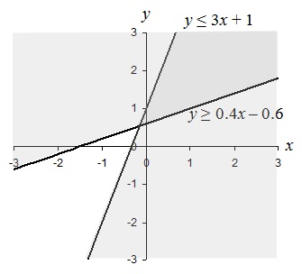
We can see in the graph that there are two shaded regions corresponding to the solutions to each inequality. The lines are shaded because the inequalities are not strict (≥ and ≤ are used). The solution to the system of inequalities is the darker shaded region, which is the overlap of the two individual regions, and the portions of the lines (rays) that border the region. Symbolically, we can perhaps best express the solution in this case as
0.4 x – 0.6 ≤ y ≤ 3 x + 1
Solving systems of inequalities in three or more dimensions is possible, but it is much more complicated-graphing the solid regions that constitute the solutions is likewise tougher.
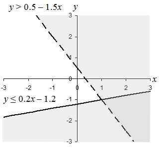
Practice Problem: Find and graph the solution set of the following system of inequalities:
x – 5 y ≥ 6
3 x + 2 y > 1
Solution : First, let's solve the expressions for y .
x – 5 y ≥ 6 3 x + 2 y > 1
x ≥ 6 + 5 y 2 y > 1 – 3 x
5 y ≤ x – 6 y > 0.5 – 1.5 x
y ≤ 0.2 x – 1.2
We can then express the solution to this system of inequalities as follows:
0.5 – 1.5 x < y ≤ 0.2 x – 1.2
Let's graph the solution set. First, we'll graph the lines corresponding to the two individual inequalities (and choosing a solid line for the first and a broken line for the second), then we'll shade the two regions appropriately.
Linear Optimization
We can apply what we have learned above to linear optimization (also called linear programming ), which is the process of finding a maximum or minimum value for some function under certain conditions (such as linear inequalities). Dealing with problems that involve linear optimization do not require you to learn any new skills; they simply require that you apply what you already know. So, let's move right to a practice problem.
Practice Problem: Find the maximum value of y given –3 x + 2 y ≤ 4 and x + y ≤ 1 subject to the condition that x ≥ 0.
Solution: What we are given is a system of inequalities for which we must first find a corresponding solution set. Within this solution set, we can then find the maximum value of y . So, we can first apply what we already know: let's rearrange the inequalities into a form that we can easily graph.
–3 x + 2 y ≤ 4 x + y ≤ 1 x ≥ 0
2 y ≤ 3 x + 4 y ≤ 1 – x
y ≤ 1.5 x + 2
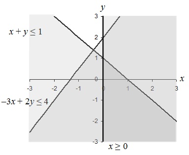
The darkest shaded region (the wedge in the lower right of the graph) satisfies all the constraints on the problem. We then want to find the maximum value of y , which is clearly 1. (We can also find this value by substituting x = 0 into x + y ≤ 1 and finding the maximum value of y , which likewise is clearly 1.)

- Course Catalog
- Group Discounts
- Gift Certificates
- For Libraries
- CEU Verification
- Medical Terminology
- Accounting Course
- Writing Basics
- QuickBooks Training
- Proofreading Class
- Sensitivity Training
- Excel Certificate
- Teach Online
- Terms of Service
- Privacy Policy

Free Mathematics Tutorials
- Math Problems
- Algebra Questions and Problems
- Graphs of Functions, Equations, and Algebra
- Free Math Worksheets to Download
- Analytical Tutorials
- Solving Equation and Inequalities
- Online Math Calculators and Solvers
- Free Graph Paper
- Math Software
- The Applications of Mathematics in Physics and Engineering
- Exercises de Mathematiques Utilisant les Applets
- Calculus Tutorials and Problems
- Calculus Questions With Answers
- Free Calculus Worksheets to Download
- Geometry Tutorials and Problems
- Online Geometry Calculators and Solvers
- Free Geometry Worksheets to Download
- Trigonometry Tutorials and Problems for Self Tests
- Free Trigonometry Questions with Answers
- Free Trigonometry Worksheets to Download
- Elementary Statistics and Probability Tutorials and Problems
- Mathematics pages in French
- About the author
- Primary Math
- Middle School Math
- High School Math
- Free Practice for SAT, ACT and Compass Math tests
Solve Systems of Inequalities with Two Variables
This is a tutorial on solving systems of inequalities with two variables . Examples with detailed explanations are presented.
In order to solve a system of inequalities, we first solve graphically each inequality in the given system on the same coordinate system and then find the region that is common to each solution (which is a region) of the inequality in the system: it is the intersection of all regions obtained and is called the feasible region.
Example 1: Solve graphically the system of inequalities
Solution to Example 1
We first use the methods developed in solving inequalities with two variables to solve each of the given inequalities in the system to solve. Below is shown (in red) the solution set of the first inequality: \( x + 2y \ge - 2 \). Because the symbol of the inequality includes the equal sign, the graph of equation \( x + 2y = - 2 \) is a solid line.
We then solve the second inequality \( x + y \lt 0 \); it is shown below in blue. Because the symbol of the inequality does not include the equal sign, the graph of the equation \( x + y = 0 \) is a broken line.
We next find the region common region to the solution sets (the intersection of the two solution set) found above. The intersection is the set of points common to the two solution sets. Shown below with both red and blue hash lines.
Finally the solution set of the system of inequalities to solve is represented by the blue region. It is called the feasible region.
Example 2 Solve graphically the inequality and find the vertices of the region representing the solution set. \[ \begin{cases} \ x \gt y - 1 \\ \ 2x + y \le 2 \\ \ 4y \ge -3 x - 12 \\ \end{cases} \]
Solution to Example 2
We first solve the inequality \( x \gt y - 1 \). The solution set is the region with black hash lines.
We then solve the inequality \( 2x + y \le 2 \). The solution set is the region with red hash lines.
We next solve the inequality \( 4y \ge -3 x - 12 \). The solution set is the region with blue hash lines.
The solution set is the intersection of all three regions found above. It is shown below as a triangle.
Finally the solution set as a triangle also called the feasible region is shown below.
Now that we have the region representing the solution set which is a triangle, we are asked to find the coordinates of the vertices A, B and C which are points of intersection of the lines graphed to find the solution set of the system of inequalities.
Point A is the intersection of the lines through AB and AC equation of line through AB: x = y - 1 equation of line through AC: 4y = - 3 x - 12 The point of intersection of AB and AC is the solution to the system of equations \[ \begin{cases} \ x = y - 1 \\ \ 4y = -3 x - 12 \\ \end{cases} \] Solve the above system to find y = - 9 / 7 and x = - 16 / 7. Point A has the coordinates: A( - 16 / 7 , - 9 / 7)
Point B is the intersection of AB and BC and is found by solving the system of equation \[ \begin{cases} \ x = y - 1 \\ \ 2x + y = 2 \\ \end{cases} \] Solution: B(1 / 3 , 4 / 3)
Point C is the intersection of AC and BC and is found by solving the system of equation \[ \begin{cases} \ 4y = -3 x - 12 \\ \ 2x + y = 2 \\ \end{cases} \] Solution: C(4 , -6)
Example 3 Solve graphically the inequality and find the vertices of the region representing the solution set. \[ \begin{cases} \ x \ge 0 \\ \ y \ge 0 \\ \ y \le x + 1 \\ \ 4y + x \le 10 \\ \ y - x \ge - 3 \\ \end{cases} \]
Solution to Example 3
We first solve each inequality and then determine the common region which is the solution set to the given system of inequalities as shown below by a polygon. This is called the feasible region. There are 5 vertices: A, B, C, D and E. Each point is determined by solving the 2 by 2 system of equations corresponding to the two lines whose intersection is the vertex to be found (see example 2 above). Point A is the intersection of lines x = 0 and y = 0. Solution A(0 , 0). Point B is is the intersection of lines x = 0 and y = x + 1. Solution B(0 , 1) Point C is is the intersection of lines y = x + 1 and 4 y + x = 10. Solution C(6/5 , 11/5) Point D is is the intersection of lines 4y + x = 10 and y - x = - 3. Solution D(22/5 , 7/5) Point E is is the intersection of lines y - x = -3 and y = 0. Solution E( 3 , 0)
POPULAR PAGES
privacy policy
A free service from Mattecentrum
Linear inequalities in two variables
- Linear inequalities with two variables I
- Linear inequalities with two variables II
- Linear inequalities with two variables III
The solution of a linear inequality in two variables like Ax + By > C is an ordered pair (x, y) that produces a true statement when the values of x and y are substituted into the inequality.
Is (1, 2) a solution to the inequality
$$2x+3y>1$$
$$2\cdot 1+3\cdot 2\overset{?}{>}1$$
$$2+5\overset{?}{>}1$$
The graph of an inequality in two variables is the set of points that represents all solutions to the inequality. A linear inequality divides the coordinate plane into two halves by a boundary line where one half represents the solutions of the inequality. The boundary line is dashed for > and < and solid for ≤ and ≥. The half-plane that is a solution to the inequality is usually shaded.
Graph the inequality
$$y\geq -x+1$$

Video lesson
Graph the linear inequality
$$y \geq 2x -3$$
- Graphing linear systems
- The substitution method for solving linear systems
- The elimination method for solving linear systems
- Systems of linear inequalities
- Properties of exponents
- Scientific notation
- Exponential growth functions
- Monomials and polynomials
- Special products of polynomials
- Polynomial equations in factored form
- Use graphing to solve quadratic equations
- Completing the square
- The quadratic formula
- The graph of a radical function
- Simplify radical expressions
- Radical equations
- The Pythagorean Theorem
- The distance and midpoint formulas
- Simplify rational expression
- Multiply rational expressions
- Division of polynomials
- Add and subtract rational expressions
- Solving rational equations
- Algebra 2 Overview
- Geometry Overview
- SAT Overview
- ACT Overview
Systems of Linear Inequalities, Word Problems - Examples - Expii
SOLVING LINEAR INEQUALITIES WORD PROBLEMS IN TWO VARIABLES
A statement involving the symbols ‘>’, ‘<’, ‘ ≥’, ‘≤’ is called an inequality.
By understanding the real situation, we have to use two variables to represent each quantities
Problem 1 :
Katie has $50 in a savings account at the beginning of the summer. She wants to have at least $20 in the account by the end of the summer. She withdraws $2 each week for food, clothes, and movie tickets. Write an inequality that expresses Katie’s situation and display it on the graph below. For how many weeks can Katie withdraw money?
Let x be the number of weeks
50 - 2x ≥ 20
2x ≤ 30
x ≤ 15 weeks

Problem 2 :
Skate Land charges a $50 flat fee for a birthday party rental and $4 for each person. Joann has no more than $100 to budget for her party. Write an inequality that models her situation and display it on the graph below. How many people can attend Joann's party.
Assume x people can attend the party.
y = 50 + 4x
50 + 4x ≤ 100
So, 12 people can attend Joan’s party.
Problem 3 :
Sarah is selling bracelets and earrings to make money for summer vacation. The bracelets cost $2 and the earrings cost $3. She needs to make at least $60. Sarah knows she will sell more than 10 bracelets. Write inequalities to represent the income from jewelry sold and number of bracelets sold. Find two possible solutions.
Let x be the number of bracelets sold.
Let y be the number of earrings sold.
2x + 3y ≥ 60
If x = 11, then 2(11) + 3y ≥ 60
3y ≥ 60 - 22
3y ≥ 38
Since y is the number of earrings, x = 11 is not possible.
| If x = 12 2(12) + 3y = 60 24 + 3y = 60 3y = 60 - 24 3y = 36 y = 12 x = 12 and y = 12 | If x = 15 2(15) + 3y = 60 30 + 3y = 60 3y = 60 - 30 3y = 30 y = 10 x = 15 and y = 10 |
- Variables and Expressions
- Variables and Expressions Worksheet
- Place Value of Number
- Formation of Large Numbers
- Laws of Exponents
- Angle Bisector Theorem
- Pre Algebra
- SAT Practice Topic Wise
- Geometry Topics
- SMO Past papers
- Parallel Lines and Angles
- Properties of Quadrilaterals
- Circles and Theorems
- Transformations of 2D Shapes
- Quadratic Equations and Functions
- Composition of Functions
- Polynomials
- Fractions Decimals and Percentage
- Customary Unit and Metric Unit
- Honors Geometry
- 8th grade worksheets
- Linear Equations
- Precalculus Worksheets
- 7th Grade Math Worksheets
- Vocabulary of Triangles and Special right triangles
- 6th Grade Math Topics
- STAAR Math Practice
- Math 1 EOC Review Worksheets
- 11 Plus Math Papers
- CA Foundation Papers
- Algebra 1 Worksheets
Recent Articles
Finding range of values inequality problems.
May 21, 24 08:51 PM
Solving Two Step Inequality Word Problems
May 21, 24 08:51 AM
Exponential Function Context and Data Modeling
May 20, 24 10:45 PM
© All rights reserved. intellectualmath.com
Grade 8 Mathematics Module: “Solving Problems Involving Linear Inequalities in Two Variables”
This Self-Learning Module (SLM) is prepared so that you, our dear learners, can continue your studies and learn while at home. Activities, questions, directions, exercises, and discussions are carefully stated for you to understand each lesson.
Each SLM is composed of different parts. Each part shall guide you step-by-step as you discover and understand the lesson prepared for you.
Pre-tests are provided to measure your prior knowledge on lessons in each SLM. This will tell you if you need to proceed on completing this module or if you need to ask your facilitator or your teacher’s assistance for better understanding of the lesson. At the end of each module, you need to answer the post-test to self-check your learning. Answer keys are provided for each activity and test. We trust that you will be honest in using these.
Please use this module with care. Do not put unnecessary marks on any part of this SLM. Use a separate sheet of paper in answering the exercises and tests. And read the instructions carefully before performing each task.
If you have any questions in using this SLM or any difficulty in answering the tasks in this module, do not hesitate to consult your teacher or facilitator.
In this module, you will be acquainted with key concepts of solving problems involving linear inequalities in two variables. You are given the opportunity to use your prior knowledge and skills in translating mathematical expressions to verbal phrase and vice-versa, then solve problems involving real-life situations. The lesson is arranged accordingly to suit to your learning needs.
This module contains:
Lesson 1- Solving Problems Involving Linear Inequalities in Two Variables
After going through this module, you are expected to:
1. translate statements into mathematical expressions.
2. solve problems involving linear inequalities in two variables; and
3. apply linear inequalities in two variables in real-life situation.
Grade 8 Mathematics Quarter 2 Self-Learning Module: “Solving Problems Involving Linear Inequalities in Two Variables”
Can't find what you're looking for.
We are here to help - please use the search box below.
2 thoughts on “Grade 8 Mathematics Module: “Solving Problems Involving Linear Inequalities in Two Variables””
Hello. I’m a Math teacher at Bayambang National HighSchool, and I would really appreciate having the answer keys to this module be posted for I have lost access to it. Thanks, Admin.
Leave a Comment Cancel reply
COMMENTS
To solve systems of linear inequalities, graph the solution sets of each inequality on the same set of axes and determine where they intersect. Exercise 4.5.1 4.5. 1 Solving Systems of Linear Inequalities. Determine whether the given point is a solution to the given system of linear equations. (3, 2) ( 3, 2); {y y ≤ x + 3 ≥ −x + 3 { y ≤ ...
Answer. ( − 3, 3) is not a solution; it does not satisfy both inequalities. We can graph the solutions of systems that contain nonlinear inequalities in a similar manner. For example, both solution sets of the following inequalities can be graphed on the same set of axes: {y < 1 2x + 4 y ≥ x2. Figure 3.7.4.
In Systems of Linear Equations in Two Variables, we learned how to solve for systems of linear equations in two variables and found a solution that would work in both equations. We can solve systems of inequalities by graphing each inequality (as discussed in Graphing Linear Equations and Inequalities) and putting these on the same coordinate ...
‼️second quarter‼️🟡 grade 8: solving problems involving systems of linear inequalities in two variables🟡 grade 8 playlistfirst quarter: https://tinyurl.co...
Shade in the side of the boundary line where the inequality is true. Step 2: On the same grid, graph the second inequality. Graph the boundary line. Shade in the side of that boundary line where the inequality is true. Step 3: The solution is the region where the shading overlaps.
2.1 Use a General Strategy to Solve Linear Equations; 2.2 Use a Problem Solving Strategy; ... 3.4 Graph Linear Inequalities in Two Variables; 3.5 Relations and Functions; 3.6 Graphs of Functions; Chapter Review. ... when we solve a system of two linear equations represented by a graph of two lines in the same plane, there are three possible ...
The graphical method of solving the system of inequalities involves the following steps. Step 1: Plot all the lines of inequalities for the given system of linear inequalities, i.e. two or more inequalities on the same Cartesian plane. Step 2: If inequality is of the type ax + by ≥ c or ax + by ≤ c, then the points on the line ax + by = c ...
This topic covers: Solutions to linear inequalities and systems of inequalities. Graphing linear inequalities and systems of inequalities. Linear inequalities and systems of inequalities word problems. Testing solutions to systems of inequalities. Constraining solutions of systems of inequalities.
Two-variable inequalities word problems. Wang Hao wants to spend at most $ 15 on dairy products. Each liter of goat milk costs $ 2.40 , and each liter of cow's milk costs $ 1.20 . Write an inequality that represents the number of liters of goat milk ( G) and cow's milk ( C) Wang Hao can buy on his budget. Learn for free about math, art ...
Solutions to a system of linear inequalities are the ordered pairs that solve all the inequalities in the system. Therefore, to solve these systems, graph the solution sets of the inequalities on the same set of axes and determine where they intersect. This intersection, or overlap, defines the region of common ordered pair solutions.
In this video you will learn how Systems of Linear Inequalities in Two Variables apply in real life situations#enjoymath #lovemath #systemoflinearinequalities
Perhaps the most lucid way to simultaneously solve a set of linear inequalities is through the use of graphs. Let's consider an example in two dimensions right away. 2x - 5y ≤ 3. y - 3x ≤ 1. Because of the inequality, we cannot use substitution in the same way as we did with systems of linear equations. Let's take a look at the graphs ...
Solution to Example 1. We first use the methods developed in solving inequalities with two variables to solve each of the given inequalities in the system to solve. Below is shown (in red) the solution set of the first inequality: x + 2y ≥ −2 x + 2 y ≥ − 2. Because the symbol of the inequality includes the equal sign, the graph of ...
y = 5. 2y = 5 is the ordered pair (1, 3). To solve a system of linear equations in two variables by the elimination method, the following procedures could be followed: ecessary, rewrite both equations in standard form Ax + By = C.Whenever necessary, multiply either equation or both equations by a nonzer.
A linear inequality divides the coordinate plane into two halves by a boundary line where one half represents the solutions of the inequality. The boundary line is dashed for > and < and solid for ≤ and ≥. The half-plane that is a solution to the inequality is usually shaded. Example. Graph the inequality. y ≥ −x + 1 y ≥ − x + 1.
So, we can say that: x+y=20. Therefore, our system of linear equations is: 50x+45y≥500 x+y=20. Step 2: Solve the inequalities. Let's solve these inequalities by graphing. Here is a graph of the two inequalities. Made using Desmos. 50x+45y≥500 is represented by the red shading. x+y=20 is represented by the blue shading.
Sarah knows she will sell more than 10 bracelets. Write inequalities to represent the income from jewelry sold and number of bracelets sold. Find two possible solutions. Solution : Let x be the number of bracelets sold. Let y be the number of earrings sold. 2x + 3y ≥ 60. x > 10. If x = 11, then 2 (11) + 3y ≥ 60.
Step 5. Solve the inequality. Step 6. Check the answer in the problem and make sure it makes sense. We substitute 27 into the inequality. 905 ≤ 500 + 15h 905 ≤ 500 + 15(27) 905 ≤ 905 Step 7. Answer the the question with a complete sentence. the number of hours Brenda must babysit Let h = the number of hours.
Lesson 1- Solving Problems Involving Linear Inequalities in Two Variables. After going through this module, you are expected to: 1. translate statements into mathematical expressions. 2. solve problems involving linear inequalities in two variables; and. 3. apply linear inequalities in two variables in real-life situation.
The method of solving linear inequalities in two variables is the same as solving linear equations. For example, if 2x + 3y > 4 is a linear inequality, then we can check the solution, by putting the values of x and y here. Let x = 1 and y = 2. Taking LHS, we have; 2 (1) + 3 (2) = 2 + 6 = 8. Since, 8 > 4, therefore, the ordered pair (1, 2 ...
This document provides a semi-detailed lesson plan on problem solving involving systems of linear inequalities in two variables. The objectives are for students to be able to identify regions representing solutions to systems of inequalities on graphs, sketch graphs representing systems, and identify systems represented by graphs. The lesson plan outlines prerequisites, exclusions, topics ...
A. Anirach Ytirahc. This document discusses solving problems involving linear inequalities in two variables. It begins by stating the learning objectives, which are to solve such problems and appreciate their use in real-life situations. An activity is presented involving using a budget to purchase ingredients for chicken adobo.
A System of Linear Inequalities in two variables consists of at least two linear inequalities. "Solving" systems of linear inequalities means "graphing each individual inequality, then finding the solution sets or group of points which satisfy all the given inequalities". The solution sets of a system of linear inequalities in two variables ...
Solving equationsMath exercises & math problems: systems of linear equations and Equations linear math systems inequalities problems solve exercises system solving two algebra exercise variables solution grade checkSolving a word problem with two unknowns using a linear equation.