stock market trading research paper

• Open access
• Published: 28 August 2020

Short-term stock market price trend prediction using a comprehensive deep learning system

• Jingyi Shen 1 &
• M. Omair Shafiq   ORCID: orcid.org/0000-0002-1859-8296 1  

Journal of Big Data volume  7 , Article number:  66 ( 2020 ) Cite this article

267k Accesses

161 Citations

91 Altmetric

Metrics details

In the era of big data, deep learning for predicting stock market prices and trends has become even more popular than before. We collected 2 years of data from Chinese stock market and proposed a comprehensive customization of feature engineering and deep learning-based model for predicting price trend of stock markets. The proposed solution is comprehensive as it includes pre-processing of the stock market dataset, utilization of multiple feature engineering techniques, combined with a customized deep learning based system for stock market price trend prediction. We conducted comprehensive evaluations on frequently used machine learning models and conclude that our proposed solution outperforms due to the comprehensive feature engineering that we built. The system achieves overall high accuracy for stock market trend prediction. With the detailed design and evaluation of prediction term lengths, feature engineering, and data pre-processing methods, this work contributes to the stock analysis research community both in the financial and technical domains.

Introduction

Stock market is one of the major fields that investors are dedicated to, thus stock market price trend prediction is always a hot topic for researchers from both financial and technical domains. In this research, our objective is to build a state-of-art prediction model for price trend prediction, which focuses on short-term price trend prediction.

As concluded by Fama in [ 26 ], financial time series prediction is known to be a notoriously difficult task due to the generally accepted, semi-strong form of market efficiency and the high level of noise. Back in 2003, Wang et al. in [ 44 ] already applied artificial neural networks on stock market price prediction and focused on volume, as a specific feature of stock market. One of the key findings by them was that the volume was not found to be effective in improving the forecasting performance on the datasets they used, which was S&P 500 and DJI. Ince and Trafalis in [ 15 ] targeted short-term forecasting and applied support vector machine (SVM) model on the stock price prediction. Their main contribution is performing a comparison between multi-layer perceptron (MLP) and SVM then found that most of the scenarios SVM outperformed MLP, while the result was also affected by different trading strategies. In the meantime, researchers from financial domains were applying conventional statistical methods and signal processing techniques on analyzing stock market data.

The optimization techniques, such as principal component analysis (PCA) were also applied in short-term stock price prediction [ 22 ]. During the years, researchers are not only focused on stock price-related analysis but also tried to analyze stock market transactions such as volume burst risks, which expands the stock market analysis research domain broader and indicates this research domain still has high potential [ 39 ]. As the artificial intelligence techniques evolved in recent years, many proposed solutions attempted to combine machine learning and deep learning techniques based on previous approaches, and then proposed new metrics that serve as training features such as Liu and Wang [ 23 ]. This type of previous works belongs to the feature engineering domain and can be considered as the inspiration of feature extension ideas in our research. Liu et al. in [ 24 ] proposed a convolutional neural network (CNN) as well as a long short-term memory (LSTM) neural network based model to analyze different quantitative strategies in stock markets. The CNN serves for the stock selection strategy, automatically extracts features based on quantitative data, then follows an LSTM to preserve the time-series features for improving profits.

The latest work also proposes a similar hybrid neural network architecture, integrating a convolutional neural network with a bidirectional long short-term memory to predict the stock market index [ 4 ]. While the researchers frequently proposed different neural network solution architectures, it brought further discussions about the topic if the high cost of training such models is worth the result or not.

There are three key contributions of our work (1) a new dataset extracted and cleansed (2) a comprehensive feature engineering, and (3) a customized long short-term memory (LSTM) based deep learning model.

We have built the dataset by ourselves from the data source as an open-sourced data API called Tushare [ 43 ]. The novelty of our proposed solution is that we proposed a feature engineering along with a fine-tuned system instead of just an LSTM model only. We observe from the previous works and find the gaps and proposed a solution architecture with a comprehensive feature engineering procedure before training the prediction model. With the success of feature extension method collaborating with recursive feature elimination algorithms, it opens doors for many other machine learning algorithms to achieve high accuracy scores for short-term price trend prediction. It proved the effectiveness of our proposed feature extension as feature engineering. We further introduced our customized LSTM model and further improved the prediction scores in all the evaluation metrics. The proposed solution outperformed the machine learning and deep learning-based models in similar previous works.

The remainder of this paper is organized as follows. “ Survey of related works ” section describes the survey of related works. “ The dataset ” section provides details on the data that we extracted from the public data sources and the dataset prepared. “ Methods ” section presents the research problems, methods, and design of the proposed solution. Detailed technical design with algorithms and how the model implemented are also included in this section. “ Results ” section presents comprehensive results and evaluation of our proposed model, and by comparing it with the models used in most of the related works. “ Discussion ” section provides a discussion and comparison of the results. “ Conclusion ” section presents the conclusion. This research paper has been built based on Shen [ 36 ].

Survey of related works

In this section, we discuss related works. We reviewed the related work in two different domains: technical and financial, respectively.

Kim and Han in [ 19 ] built a model as a combination of artificial neural networks (ANN) and genetic algorithms (GAs) with discretization of features for predicting stock price index. The data used in their study include the technical indicators as well as the direction of change in the daily Korea stock price index (KOSPI). They used the data containing samples of 2928 trading days, ranging from January 1989 to December 1998, and give their selected features and formulas. They also applied optimization of feature discretization, as a technique that is similar to dimensionality reduction. The strengths of their work are that they introduced GA to optimize the ANN. First, the amount of input features and processing elements in the hidden layer are 12 and not adjustable. Another limitation is in the learning process of ANN, and the authors only focused on two factors in optimization. While they still believed that GA has great potential for feature discretization optimization. Our initialized feature pool refers to the selected features. Qiu and Song in [ 34 ] also presented a solution to predict the direction of the Japanese stock market based on an optimized artificial neural network model. In this work, authors utilize genetic algorithms together with artificial neural network based models, and name it as a hybrid GA-ANN model.

Piramuthu in [ 33 ] conducted a thorough evaluation of different feature selection methods for data mining applications. He used for datasets, which were credit approval data, loan defaults data, web traffic data, tam, and kiang data, and compared how different feature selection methods optimized decision tree performance. The feature selection methods he compared included probabilistic distance measure: the Bhattacharyya measure, the Matusita measure, the divergence measure, the Mahalanobis distance measure, and the Patrick-Fisher measure. For inter-class distance measures: the Minkowski distance measure, city block distance measure, Euclidean distance measure, the Chebychev distance measure, and the nonlinear (Parzen and hyper-spherical kernel) distance measure. The strength of this paper is that the author evaluated both probabilistic distance-based and several inter-class feature selection methods. Besides, the author performed the evaluation based on different datasets, which reinforced the strength of this paper. However, the evaluation algorithm was a decision tree only. We cannot conclude if the feature selection methods will still perform the same on a larger dataset or a more complex model.

Hassan and Nath in [ 9 ] applied the Hidden Markov Model (HMM) on the stock market forecasting on stock prices of four different Airlines. They reduce states of the model into four states: the opening price, closing price, the highest price, and the lowest price. The strong point of this paper is that the approach does not need expert knowledge to build a prediction model. While this work is limited within the industry of Airlines and evaluated on a very small dataset, it may not lead to a prediction model with generality. One of the approaches in stock market prediction related works could be exploited to do the comparison work. The authors selected a maximum 2 years as the date range of training and testing dataset, which provided us a date range reference for our evaluation part.

Lei in [ 21 ] exploited Wavelet Neural Network (WNN) to predict stock price trends. The author also applied Rough Set (RS) for attribute reduction as an optimization. Rough Set was utilized to reduce the stock price trend feature dimensions. It was also used to determine the structure of the Wavelet Neural Network. The dataset of this work consists of five well-known stock market indices, i.e., (1) SSE Composite Index (China), (2) CSI 300 Index (China), (3) All Ordinaries Index (Australian), (4) Nikkei 225 Index (Japan), and (5) Dow Jones Index (USA). Evaluation of the model was based on different stock market indices, and the result was convincing with generality. By using Rough Set for optimizing the feature dimension before processing reduces the computational complexity. However, the author only stressed the parameter adjustment in the discussion part but did not specify the weakness of the model itself. Meanwhile, we also found that the evaluations were performed on indices, the same model may not have the same performance if applied on a specific stock.

Lee in [ 20 ] used the support vector machine (SVM) along with a hybrid feature selection method to carry out prediction of stock trends. The dataset in this research is a sub dataset of NASDAQ Index in Taiwan Economic Journal Database (TEJD) in 2008. The feature selection part was using a hybrid method, supported sequential forward search (SSFS) played the role of the wrapper. Another advantage of this work is that they designed a detailed procedure of parameter adjustment with performance under different parameter values. The clear structure of the feature selection model is also heuristic to the primary stage of model structuring. One of the limitations was that the performance of SVM was compared to back-propagation neural network (BPNN) only and did not compare to the other machine learning algorithms.

Sirignano and Cont leveraged a deep learning solution trained on a universal feature set of financial markets in [ 40 ]. The dataset used included buy and sell records of all transactions, and cancellations of orders for approximately 1000 NASDAQ stocks through the order book of the stock exchange. The NN consists of three layers with LSTM units and a feed-forward layer with rectified linear units (ReLUs) at last, with stochastic gradient descent (SGD) algorithm as an optimization. Their universal model was able to generalize and cover the stocks other than the ones in the training data. Though they mentioned the advantages of a universal model, the training cost was still expensive. Meanwhile, due to the inexplicit programming of the deep learning algorithm, it is unclear that if there are useless features contaminated when feeding the data into the model. Authors found out that it would have been better if they performed feature selection part before training the model and found it as an effective way to reduce the computational complexity.

Ni et al. in [ 30 ] predicted stock price trends by exploiting SVM and performed fractal feature selection for optimization. The dataset they used is the Shanghai Stock Exchange Composite Index (SSECI), with 19 technical indicators as features. Before processing the data, they optimized the input data by performing feature selection. When finding the best parameter combination, they also used a grid search method, which is k cross-validation. Besides, the evaluation of different feature selection methods is also comprehensive. As the authors mentioned in their conclusion part, they only considered the technical indicators but not macro and micro factors in the financial domain. The source of datasets that the authors used was similar to our dataset, which makes their evaluation results useful to our research. They also mentioned a method called k cross-validation when testing hyper-parameter combinations.

McNally et al. in [ 27 ] leveraged RNN and LSTM on predicting the price of Bitcoin, optimized by using the Boruta algorithm for feature engineering part, and it works similarly to the random forest classifier. Besides feature selection, they also used Bayesian optimization to select LSTM parameters. The Bitcoin dataset ranged from the 19th of August 2013 to 19th of July 2016. Used multiple optimization methods to improve the performance of deep learning methods. The primary problem of their work is overfitting. The research problem of predicting Bitcoin price trend has some similarities with stock market price prediction. Hidden features and noises embedded in the price data are threats of this work. The authors treated the research question as a time sequence problem. The best part of this paper is the feature engineering and optimization part; we could replicate the methods they exploited in our data pre-processing.

Weng et al. in [ 45 ] focused on short-term stock price prediction by using ensemble methods of four well-known machine learning models. The dataset for this research is five sets of data. They obtained these datasets from three open-sourced APIs and an R package named TTR. The machine learning models they used are (1) neural network regression ensemble (NNRE), (2) a Random Forest with unpruned regression trees as base learners (RFR), (3) AdaBoost with unpruned regression trees as base learners (BRT) and (4) a support vector regression ensemble (SVRE). A thorough study of ensemble methods specified for short-term stock price prediction. With background knowledge, the authors selected eight technical indicators in this study then performed a thoughtful evaluation of five datasets. The primary contribution of this paper is that they developed a platform for investors using R, which does not need users to input their own data but call API to fetch the data from online source straightforward. From the research perspective, they only evaluated the prediction of the price for 1 up to 10 days ahead but did not evaluate longer terms than two trading weeks or a shorter term than 1 day. The primary limitation of their research was that they only analyzed 20 U.S.-based stocks, the model might not be generalized to other stock market or need further revalidation to see if it suffered from overfitting problems.

Kara et al. in [ 17 ] also exploited ANN and SVM in predicting the movement of stock price index. The data set they used covers a time period from January 2, 1997, to December 31, 2007, of the Istanbul Stock Exchange. The primary strength of this work is its detailed record of parameter adjustment procedures. While the weaknesses of this work are that neither the technical indicator nor the model structure has novelty, and the authors did not explain how their model performed better than other models in previous works. Thus, more validation works on other datasets would help. They explained how ANN and SVM work with stock market features, also recorded the parameter adjustment. The implementation part of our research could benefit from this previous work.

Jeon et al. in [ 16 ] performed research on millisecond interval-based big dataset by using pattern graph tracking to complete stock price prediction tasks. The dataset they used is a millisecond interval-based big dataset of historical stock data from KOSCOM, from August 2014 to October 2014, 10G–15G capacity. The author applied Euclidean distance, Dynamic Time Warping (DTW) for pattern recognition. For feature selection, they used stepwise regression. The authors completed the prediction task by ANN and Hadoop and RHive for big data processing. The “ Results ” section is based on the result processed by a combination of SAX and Jaro–Winkler distance. Before processing the data, they generated aggregated data at 5-min intervals from discrete data. The primary strength of this work is the explicit structure of the whole implementation procedure. While they exploited a relatively old model, another weakness is the overall time span of the training dataset is extremely short. It is difficult to access the millisecond interval-based data in real life, so the model is not as practical as a daily based data model.

Huang et al. in [ 12 ] applied a fuzzy-GA model to complete the stock selection task. They used the key stocks of the 200 largest market capitalization listed as the investment universe in the Taiwan Stock Exchange. Besides, the yearly financial statement data and the stock returns were taken from the Taiwan Economic Journal (TEJ) database at www.tej.com.tw/ for the time period from year 1995 to year 2009. They conducted the fuzzy membership function with model parameters optimized with GA and extracted features for optimizing stock scoring. The authors proposed an optimized model for selection and scoring of stocks. Different from the prediction model, the authors more focused on stock rankings, selection, and performance evaluation. Their structure is more practical among investors. But in the model validation part, they did not compare the model with existed algorithms but the statistics of the benchmark, which made it challenging to identify if GA would outperform other algorithms.

Fischer and Krauss in [ 5 ] applied long short-term memory (LSTM) on financial market prediction. The dataset they used is S&P 500 index constituents from Thomson Reuters. They obtained all month-end constituent lists for the S&P 500 from Dec 1989 to Sep 2015, then consolidated the lists into a binary matrix to eliminate survivor bias. The authors also used RMSprop as an optimizer, which is a mini-batch version of rprop. The primary strength of this work is that the authors used the latest deep learning technique to perform predictions. They relied on the LSTM technique, lack of background knowledge in the financial domain. Although the LSTM outperformed the standard DNN and logistic regression algorithms, while the author did not mention the effort to train an LSTM with long-time dependencies.

Tsai and Hsiao in [ 42 ] proposed a solution as a combination of different feature selection methods for prediction of stocks. They used Taiwan Economic Journal (TEJ) database as data source. The data used in their analysis was from year 2000 to 2007. In their work, they used a sliding window method and combined it with multi layer perceptron (MLP) based artificial neural networks with back propagation, as their prediction model. In their work, they also applied principal component analysis (PCA) for dimensionality reduction, genetic algorithms (GA) and the classification and regression trees (CART) to select important features. They did not just rely on technical indices only. Instead, they also included both fundamental and macroeconomic indices in their analysis. The authors also reported a comparison on feature selection methods. The validation part was done by combining the model performance stats with statistical analysis.

Pimenta et al. in [ 32 ] leveraged an automated investing method by using multi-objective genetic programming and applied it in the stock market. The dataset was obtained from Brazilian stock exchange market (BOVESPA), and the primary techniques they exploited were a combination of multi-objective optimization, genetic programming, and technical trading rules. For optimization, they leveraged genetic programming (GP) to optimize decision rules. The novelty of this paper was in the evaluation part. They included a historical period, which was a critical moment of Brazilian politics and economics when performing validation. This approach reinforced the generalization strength of their proposed model. When selecting the sub-dataset for evaluation, they also set criteria to ensure more asset liquidity. While the baseline of the comparison was too basic and fundamental, and the authors did not perform any comparison with other existing models.

Huang and Tsai in [ 13 ] conducted a filter-based feature selection assembled with a hybrid self-organizing feature map (SOFM) support vector regression (SVR) model to forecast Taiwan index futures (FITX) trend. They divided the training samples into clusters to marginally improve the training efficiency. The authors proposed a comprehensive model, which was a combination of two novel machine learning techniques in stock market analysis. Besides, the optimizer of feature selection was also applied before the data processing to improve the prediction accuracy and reduce the computational complexity of processing daily stock index data. Though they optimized the feature selection part and split the sample data into small clusters, it was already strenuous to train daily stock index data of this model. It would be difficult for this model to predict trading activities in shorter time intervals since the data volume would be increased drastically. Moreover, the evaluation is not strong enough since they set a single SVR model as a baseline, but did not compare the performance with other previous works, which caused difficulty for future researchers to identify the advantages of SOFM-SVR model why it outperforms other algorithms.

Thakur and Kumar in [ 41 ] also developed a hybrid financial trading support system by exploiting multi-category classifiers and random forest (RAF). They conducted their research on stock indices from NASDAQ, DOW JONES, S&P 500, NIFTY 50, and NIFTY BANK. The authors proposed a hybrid model combined random forest (RF) algorithms with a weighted multicategory generalized eigenvalue support vector machine (WMGEPSVM) to generate “Buy/Hold/Sell” signals. Before processing the data, they used Random Forest (RF) for feature pruning. The authors proposed a practical model designed for real-life investment activities, which could generate three basic signals for investors to refer to. They also performed a thorough comparison of related algorithms. While they did not mention the time and computational complexity of their works. Meanwhile, the unignorable issue of their work was the lack of financial domain knowledge background. The investors regard the indices data as one of the attributes but could not take the signal from indices to operate a specific stock straightforward.

Hsu in [ 11 ] assembled feature selection with a back propagation neural network (BNN) combined with genetic programming to predict the stock/futures price. The dataset in this research was obtained from Taiwan Stock Exchange Corporation (TWSE). The authors have introduced the description of the background knowledge in detail. While the weakness of their work is that it is a lack of data set description. This is a combination of the model proposed by other previous works. Though we did not see the novelty of this work, we can still conclude that the genetic programming (GP) algorithm is admitted in stock market research domain. To reinforce the validation strengths, it would be good to consider adding GP models into evaluation if the model is predicting a specific price.

Hafezi et al. in [ 7 ] built a bat-neural network multi-agent system (BN-NMAS) to predict stock price. The dataset was obtained from the Deutsche bundes-bank. They also applied the Bat algorithm (BA) for optimizing neural network weights. The authors illustrated their overall structure and logic of system design in clear flowcharts. While there were very few previous works that had performed on DAX data, it would be difficult to recognize if the model they proposed still has the generality if migrated on other datasets. The system design and feature selection logic are fascinating, which worth referring to. Their findings in optimization algorithms are also valuable for the research in the stock market price prediction research domain. It is worth trying the Bat algorithm (BA) when constructing neural network models.

Long et al. in [ 25 ] conducted a deep learning approach to predict the stock price movement. The dataset they used is the Chinese stock market index CSI 300. For predicting the stock price movement, they constructed a multi-filter neural network (MFNN) with stochastic gradient descent (SGD) and back propagation optimizer for learning NN parameters. The strength of this paper is that the authors exploited a novel model with a hybrid model constructed by different kinds of neural networks, it provides an inspiration for constructing hybrid neural network structures.

Atsalakis and Valavanis in [ 1 ] proposed a solution of a neuro-fuzzy system, which is composed of controller named as Adaptive Neuro Fuzzy Inference System (ANFIS), to achieve short-term stock price trend prediction. The noticeable strength of this work is the evaluation part. Not only did they compare their proposed system with the popular data models, but also compared with investment strategies. While the weakness that we found from their proposed solution is that their solution architecture is lack of optimization part, which might limit their model performance. Since our proposed solution is also focusing on short-term stock price trend prediction, this work is heuristic for our system design. Meanwhile, by comparing with the popular trading strategies from investors, their work inspired us to compare the strategies used by investors with techniques used by researchers.

Nekoeiqachkanloo et al. in [ 29 ] proposed a system with two different approaches for stock investment. The strengths of their proposed solution are obvious. First, it is a comprehensive system that consists of data pre-processing and two different algorithms to suggest the best investment portions. Second, the system also embedded with a forecasting component, which also retains the features of the time series. Last but not least, their input features are a mix of fundamental features and technical indices that aim to fill in the gap between the financial domain and technical domain. However, their work has a weakness in the evaluation part. Instead of evaluating the proposed system on a large dataset, they chose 25 well-known stocks. There is a high possibility that the well-known stocks might potentially share some common hidden features.

As another related latest work, Idrees et al. [ 14 ] published a time series-based prediction approach for the volatility of the stock market. ARIMA is not a new approach in the time series prediction research domain. Their work is more focusing on the feature engineering side. Before feeding the features into ARIMA models, they designed three steps for feature engineering: Analyze the time series, identify if the time series is stationary or not, perform estimation by plot ACF and PACF charts and look for parameters. The only weakness of their proposed solution is that the authors did not perform any customization on the existing ARIMA model, which might limit the system performance to be improved.

One of the main weaknesses found in the related works is limited data-preprocessing mechanisms built and used. Technical works mostly tend to focus on building prediction models. When they select the features, they list all the features mentioned in previous works and go through the feature selection algorithm then select the best-voted features. Related works in the investment domain have shown more interest in behavior analysis, such as how herding behaviors affect the stock performance, or how the percentage of inside directors hold the firm’s common stock affects the performance of a certain stock. These behaviors often need a pre-processing procedure of standard technical indices and investment experience to recognize.

In the related works, often a thorough statistical analysis is performed based on a special dataset and conclude new features rather than performing feature selections. Some data, such as the percentage of a certain index fluctuation has been proven to be effective on stock performance. We believe that by extracting new features from data, then combining such features with existed common technical indices will significantly benefit the existing and well-tested prediction models.

The dataset

This section details the data that was extracted from the public data sources, and the final dataset that was prepared. Stock market-related data are diverse, so we first compared the related works from the survey of financial research works in stock market data analysis to specify the data collection directions. After collecting the data, we defined a data structure of the dataset. Given below, we describe the dataset in detail, including the data structure, and data tables in each category of data with the segment definitions.

Description of our dataset

In this section, we will describe the dataset in detail. This dataset consists of 3558 stocks from the Chinese stock market. Besides the daily price data, daily fundamental data of each stock ID, we also collected the suspending and resuming history, top 10 shareholders, etc. We list two reasons that we choose 2 years as the time span of this dataset: (1) most of the investors perform stock market price trend analysis using the data within the latest 2 years, (2) using more recent data would benefit the analysis result. We collected data through the open-sourced API, namely Tushare [ 43 ], mean-while we also leveraged a web-scraping technique to collect data from Sina Finance web pages, SWS Research website.

Data structure

Figure  1 illustrates all the data tables in the dataset. We collected four categories of data in this dataset: (1) basic data, (2) trading data, (3) finance data, and (4) other reference data. All the data tables can be linked to each other by a common field called “Stock ID” It is a unique stock identifier registered in the Chinese Stock market. Table  1 shows an overview of the dataset.

Data structure for the extracted dataset

The Table  1 lists the field information of each data table as well as which category the data table belongs to.

In this section, we present the proposed methods and the design of the proposed solution. Moreover, we also introduce the architecture design as well as algorithmic and implementation details.

Problem statement

We analyzed the best possible approach for predicting short-term price trends from different aspects: feature engineering, financial domain knowledge, and prediction algorithm. Then we addressed three research questions in each aspect, respectively: How can feature engineering benefit model prediction accuracy? How do findings from the financial domain benefit prediction model design? And what is the best algorithm for predicting short-term price trends?

The first research question is about feature engineering. We would like to know how the feature selection method benefits the performance of prediction models. From the abundance of the previous works, we can conclude that stock price data embedded with a high level of noise, and there are also correlations between features, which makes the price prediction notoriously difficult. That is also the primary reason for most of the previous works introduced the feature engineering part as an optimization module.

The second research question is evaluating the effectiveness of findings we extracted from the financial domain. Different from the previous works, besides the common evaluation of data models such as the training costs and scores, our evaluation will emphasize the effectiveness of newly added features that we extracted from the financial domain. We introduce some features from the financial domain. While we only obtained some specific findings from previous works, and the related raw data needs to be processed into usable features. After extracting related features from the financial domain, we combine the features with other common technical indices for voting out the features with a higher impact. There are numerous features said to be effective from the financial domain, and it would be impossible for us to cover all of them. Thus, how to appropriately convert the findings from the financial domain to a data processing module of our system design is a hidden research question that we attempt to answer.

The third research question is that which algorithms are we going to model our data? From the previous works, researchers have been putting efforts into the exact price prediction. We decompose the problem into predicting the trend and then the exact number. This paper focuses on the first step. Hence, the objective has been converted to resolve a binary classification problem, meanwhile, finding an effective way to eliminate the negative effect brought by the high level of noise. Our approach is to decompose the complex problem into sub-problems which have fewer dependencies and resolve them one by one, and then compile the resolutions into an ensemble model as an aiding system for investing behavior reference.

In the previous works, researchers have been using a variety of models for predicting stock price trends. While most of the best-performed models are based on machine learning techniques, in this work, we will compare our approach with the outperformed machine learning models in the evaluation part and find the solution for this research question.

Proposed solution

The high-level architecture of our proposed solution could be separated into three parts. First is the feature selection part, to guarantee the selected features are highly effective. Second, we look into the data and perform the dimensionality reduction. And the last part, which is the main contribution of our work is to build a prediction model of target stocks. Figure  2 depicts a high-level architecture of the proposed solution.

High-level architecture of the proposed solution

There are ways to classify different categories of stocks. Some investors prefer long-term investments, while others show more interest in short-term investments. It is common to see the stock-related reports showing an average performance, while the stock price is increasing drastically; this is one of the phenomena that indicate the stock price prediction has no fixed rules, thus finding effective features before training a model on data is necessary.

In this research, we focus on the short-term price trend prediction. Currently, we only have the raw data with no labels. So, the very first step is to label the data. We mark the price trend by comparing the current closing price with the closing price of n trading days ago, the range of n is from 1 to 10 since our research is focusing on the short-term. If the price trend goes up, we mark it as 1 or mark as 0 in the opposite case. To be more specified, we use the indices from the indices of n  −  1 th day to predict the price trend of the n th day.

According to the previous works, some researchers who applied both financial domain knowledge and technical methods on stock data were using rules to filter the high-quality stocks. We referred to their works and exploited their rules to contribute to our feature extension design.

However, to ensure the best performance of the prediction model, we will look into the data first. There are a large number of features in the raw data; if we involve all the features into our consideration, it will not only drastically increase the computational complexity but will also cause side effects if we would like to perform unsupervised learning in further research. So, we leverage the recursive feature elimination (RFE) to ensure all the selected features are effective.

We found most of the previous works in the technical domain were analyzing all the stocks, while in the financial domain, researchers prefer to analyze the specific scenario of investment, to fill the gap between the two domains, we decide to apply a feature extension based on the findings we gathered from the financial domain before we start the RFE procedure.

Since we plan to model the data into time series, the number of the features, the more complex the training procedure will be. So, we will leverage the dimensionality reduction by using randomized PCA at the beginning of our proposed solution architecture.

Detailed technical design elaboration

This section provides an elaboration of the detailed technical design as being a comprehensive solution based on utilizing, combining, and customizing several existing data preprocessing, feature engineering, and deep learning techniques. Figure  3 provides the detailed technical design from data processing to prediction, including the data exploration. We split the content by main procedures, and each procedure contains algorithmic steps. Algorithmic details are elaborated in the next section. The contents of this section will focus on illustrating the data workflow.

Detailed technical design of the proposed solution

Based on the literature review, we select the most commonly used technical indices and then feed them into the feature extension procedure to get the expanded feature set. We will select the most effective i features from the expanded feature set. Then we will feed the data with i selected features into the PCA algorithm to reduce the dimension into j features. After we get the best combination of i and j , we process the data into finalized the feature set and feed them into the LSTM [ 10 ] model to get the price trend prediction result.

The novelty of our proposed solution is that we will not only apply the technical method on raw data but also carry out the feature extensions that are used among stock market investors. Details on feature extension are given in the next subsection. Experiences gained from applying and optimizing deep learning based solutions in [ 37 , 38 ] were taken into account while designing and customizing feature engineering and deep learning solution in this work.

Applying feature extension

The first main procedure in Fig.  3 is the feature extension. In this block, the input data is the most commonly used technical indices concluded from related works. The three feature extension methods are max–min scaling, polarizing, and calculating fluctuation percentage. Not all the technical indices are applicable for all three of the feature extension methods; this procedure only applies the meaningful extension methods on technical indices. We choose meaningful extension methods while looking at how the indices are calculated. The technical indices and the corresponding feature extension methods are illustrated in Table  2 .

After the feature extension procedure, the expanded features will be combined with the most commonly used technical indices, i.e., input data with output data, and feed into RFE block as input data in the next step.

Applying recursive feature elimination

After the feature extension above, we explore the most effective i features by using the Recursive Feature Elimination (RFE) algorithm [ 6 ]. We estimate all the features by two attributes, coefficient, and feature importance. We also limit the features that remove from the pool by one, which means we will remove one feature at each step and retain all the relevant features. Then the output of the RFE block will be the input of the next step, which refers to PCA.

Applying principal component analysis (PCA)

The very first step before leveraging PCA is feature pre-processing. Because some of the features after RFE are percentage data, while others are very large numbers, i.e., the output from RFE are in different units. It will affect the principal component extraction result. Thus, before feeding the data into the PCA algorithm [ 8 ], a feature pre-processing is necessary. We also illustrate the effectiveness and methods comparison in “ Results ” section.

After performing feature pre-processing, the next step is to feed the processed data with selected i features into the PCA algorithm to reduce the feature matrix scale into j features. This step is to retain as many effective features as possible and meanwhile eliminate the computational complexity of training the model. This research work also evaluates the best combination of i and j, which has relatively better prediction accuracy, meanwhile, cuts the computational consumption. The result can be found in the “ Results ” section, as well. After the PCA step, the system will get a reshaped matrix with j columns.

Fitting long short-term memory (LSTM) model

PCA reduced the dimensions of the input data, while the data pre-processing is mandatory before feeding the data into the LSTM layer. The reason for adding the data pre-processing step before the LSTM model is that the input matrix formed by principal components has no time steps. While one of the most important parameters of training an LSTM is the number of time steps. Hence, we have to model the matrix into corresponding time steps for both training and testing dataset.

After performing the data pre-processing part, the last step is to feed the training data into LSTM and evaluate the performance using testing data. As a variant neural network of RNN, even with one LSTM layer, the NN structure is still a deep neural network since it can process sequential data and memorizes its hidden states through time. An LSTM layer is composed of one or more LSTM units, and an LSTM unit consists of cells and gates to perform classification and prediction based on time series data.

The LSTM structure is formed by two layers. The input dimension is determined by j after the PCA algorithm. The first layer is the input LSTM layer, and the second layer is the output layer. The final output will be 0 or 1 indicates if the stock price trend prediction result is going down or going up, as a supporting suggestion for the investors to perform the next investment decision.

Design discussion

Feature extension is one of the novelties of our proposed price trend predicting system. In the feature extension procedure, we use technical indices to collaborate with the heuristic processing methods learned from investors, which fills the gap between the financial research area and technical research area.

Since we proposed a system of price trend prediction, feature engineering is extremely important to the final prediction result. Not only the feature extension method is helpful to guarantee we do not miss the potentially correlated feature, but also feature selection method is necessary for pooling the effective features. The more irrelevant features are fed into the model, the more noise would be introduced. Each main procedure is carefully considered contributing to the whole system design.

Besides the feature engineering part, we also leverage LSTM, the state-of-the-art deep learning method for time-series prediction, which guarantees the prediction model can capture both complex hidden pattern and the time-series related pattern.

It is known that the training cost of deep learning models is expansive in both time and hardware aspects; another advantage of our system design is the optimization procedure—PCA. It can retain the principal components of the features while reducing the scale of the feature matrix, thus help the system to save the training cost of processing the large time-series feature matrix.

Algorithm elaboration

This section provides comprehensive details on the algorithms we built while utilizing and customizing different existing techniques. Details about the terminologies, parameters, as well as optimizers. From the legend on the right side of Fig.  3 , we note the algorithm steps as octagons, all of them can be found in this “ Algorithm elaboration ” section.

Before dive deep into the algorithm steps, here is the brief introduction of data pre-processing: since we will go through the supervised learning algorithms, we also need to program the ground truth. The ground truth of this research is programmed by comparing the closing price of the current trading date with the closing price of the previous trading date the users want to compare with. Label the price increase as 1, else the ground truth will be labeled as 0. Because this research work is not only focused on predicting the price trend of a specific period of time but short-term in general, the ground truth processing is according to a range of trading days. While the algorithms will not change with the prediction term length, we can regard the term length as a parameter.

The algorithmic detail is elaborated, respectively, the first algorithm is the hybrid feature engineering part for preparing high-quality training and testing data. It corresponds to the Feature extension, RFE, and PCA blocks in Fig.  3 . The second algorithm is the LSTM procedure block, including time-series data pre-processing, NN constructing, training, and testing.

Algorithm 1: Short-term stock market price trend prediction—applying feature engineering using FE + RFE + PCA

The function FE is corresponding to the feature extension block. For the feature extension procedure, we apply three different processing methods to translate the findings from the financial domain to a technical module in our system design. While not all the indices are applicable for expanding, we only choose the proper method(s) for certain features to perform the feature extension (FE), according to Table  2 .

Normalize method preserves the relative frequencies of the terms, and transform the technical indices into the range of [0, 1]. Polarize is a well-known method often used by real-world investors, sometimes they prefer to consider if the technical index value is above or below zero, we program some of the features using polarize method and prepare for RFE. Max-min (or min-max) [ 35 ] scaling is a transformation method often used as an alternative to zero mean and unit variance scaling. Another well-known method used is fluctuation percentage, and we transform the technical indices fluctuation percentage into the range of [− 1, 1].

The function RFE () in the first algorithm refers to recursive feature elimination. Before we perform the training data scale reduction, we will have to make sure that the features we selected are effective. Ineffective features will not only drag down the classification precision but also add more computational complexity. For the feature selection part, we choose recursive feature elimination (RFE). As [ 45 ] explained, the process of recursive feature elimination can be split into the ranking algorithm, resampling, and external validation.

For the ranking algorithm, it fits the model to the features and ranks by the importance to the model. We set the parameter to retain i numbers of features, and at each iteration of feature selection retains Si top-ranked features, then refit the model and assess the performance again to begin another iteration. The ranking algorithm will eventually determine the top Si features.

The RFE algorithm is known to have suffered from the over-fitting problem. To eliminate the over-fitting issue, we will run the RFE algorithm multiple times on randomly selected stocks as the training set and ensure all the features we select are high-weighted. This procedure is called data resampling. Resampling can be built as an optimization step as an outer layer of the RFE algorithm.

The last part of our hybrid feature engineering algorithm is for optimization purposes. For the training data matrix scale reduction, we apply Randomized principal component analysis (PCA) [ 31 ], before we decide the features of the classification model.

Financial ratios of a listed company are used to present the growth ability, earning ability, solvency ability, etc. Each financial ratio consists of a set of technical indices, each time we add a technical index (or feature) will add another column of data into the data matrix and will result in low training efficiency and redundancy. If non-relevant or less relevant features are included in training data, it will also decrease the precision of classification.

The above equation represents the explanation power of principal components extracted by PCA method for original data. If an ACR is below 85%, the PCA method would be unsuitable due to a loss of original information. Because the covariance matrix is sensitive to the order of magnitudes of data, there should be a data standardize procedure before performing the PCA. The commonly used standardized methods are mean-standardization and normal-standardization and are noted as given below:

Mean-standardization: \(X_{ij}^{*} = X_{ij} /\overline{{X_{j} }}\) , which \(\overline{{X_{j} }}\) represents the mean value.

Normal-standardization: \(X_{ij}^{*} = (X_{ij} - \overline{{X_{j} }} )/s_{j}\) , which \(\overline{{X_{j} }}\) represents the mean value, and \(s_{j}\) is the standard deviation.

The array fe_array is defined according to Table  2 , row number maps to the features, columns 0, 1, 2, 3 note for the extension methods of normalize, polarize, max–min scale, and fluctuation percentage, respectively. Then we fill in the values for the array by the rule where 0 stands for no necessity to expand and 1 for features need to apply the corresponding extension methods. The final algorithm of data preprocessing using RFE and PCA can be illustrated as Algorithm 1.

Algorithm 2: Price trend prediction model using LSTM

After the principal component extraction, we will get the scale-reduced matrix, which means i most effective features are converted into j principal components for training the prediction model. We utilized an LSTM model and added a conversion procedure for our stock price dataset. The detailed algorithm design is illustrated in Alg 2. The function TimeSeriesConversion () converts the principal components matrix into time series by shifting the input data frame according to the number of time steps [ 3 ], i.e., term length in this research. The processed dataset consists of the input sequence and forecast sequence. In this research, the parameter of LAG is 1, because the model is detecting the pattern of features fluctuation on a daily basis. Meanwhile, the N_TIME_STEPS is varied from 1 trading day to 10 trading days. The functions DataPartition (), FitModel (), EvaluateModel () are regular steps without customization. The NN structure design, optimizer decision, and other parameters are illustrated in function ModelCompile () .

Some procedures impact the efficiency but do not affect the accuracy or precision and vice versa, while other procedures may affect both efficiency and prediction result. To fully evaluate our algorithm design, we structure the evaluation part by main procedures and evaluate how each procedure affects the algorithm performance. First, we evaluated our solution on a machine with 2.2 GHz i7 processor, with 16 GB of RAM. Furthermore, we also evaluated our solution on Amazon EC2 instance, 3.1 GHz Processor with 16 vCPUs, and 64 GB RAM.

In the implementation part, we expanded 20 features into 54 features, while we retain 30 features that are the most effective. In this section, we discuss the evaluation of feature selection. The dataset was divided into two different subsets, i.e., training and testing datasets. Test procedure included two parts, one testing dataset is for feature selection, and another one is for model testing. We note the feature selection dataset and model testing dataset as DS_test_f and DS_test_m, respectively.

We randomly selected two-thirds of the stock data by stock ID for RFE training and note the dataset as DS_train_f; all the data consist of full technical indices and expanded features throughout 2018. The estimator of the RFE algorithm is SVR with linear kernels. We rank the 54 features by voting and get 30 effective features then process them using the PCA algorithm to perform dimension reduction and reduce the features into 20 principal components. The rest of the stock data forms the testing dataset DS_test_f to validate the effectiveness of principal components we extracted from selected features. We reformed all the data from 2018 as the training dataset of the data model and noted as DS_train_m. The model testing dataset DS_test_m consists of the first 3 months of data in 2019, which has no overlap with the dataset we utilized in the previous steps. This approach is to prevent the hidden problem caused by overfitting.

Term length

To build an efficient prediction model, instead of the approach of modeling the data to time series, we determined to use 1 day ahead indices data to predict the price trend of the next day. We tested the RFE algorithm on a range of short-term from 1 day to 2 weeks (ten trading days), to evaluate how the commonly used technical indices correlated to price trends. For evaluating the prediction term length, we fully expanded the features as Table  2 , and feed them to RFE. During the test, we found that different length of the term has a different level of sensitive-ness to the same indices set.

We get the close price of the first trading date and compare it with the close price of the n _ th trading date. Since we are predicting the price trend, we do not consider the term lengths if the cross-validation score is below 0.5. And after the test, as we can see from Fig.  4 , there are three-term lengths that are most sensitive to the indices we selected from the related works. They are n  = {2, 5, 10}, which indicates that price trend prediction of every other day, 1 week, and 2 weeks using the indices set are likely to be more reliable.

How do term lengths affect the cross-validation score of RFE

While these curves have different patterns, for the length of 2 weeks, the cross-validation score increases with the number of features selected. If the prediction term length is 1 week, the cross-validation score will decrease if selected over 8 features. For every other day price trend prediction, the best cross-validation score is achieved by selecting 48 features. Biweekly prediction requires 29 features to achieve the best score. In Table  3 , we listed the top 15 effective features for these three-period lengths. If we predict the price trend of every other day, the cross-validation score merely fluctuates with the number of features selected. So, in the next step, we will evaluate the RFE result for these three-term lengths, as shown in Fig.  4 .

We compare the output feature set of RFE with the all-original feature set as a baseline, the all-original feature set consists of n features and we choose n most effective features from RFE output features to evaluate the result using linear SVR. We used two different approaches to evaluate feature effectiveness. The first method is to combine all the data into one large matrix and evaluate them by running the RFE algorithm once. Another method is to run RFE for each individual stock and calculate the most effective features by voting.

Feature extension and RFE

From the result of the previous subsection, we can see that when predicting the price trend for every other day or biweekly, the best result is achieved by selecting a large number of features. Within the selected features, some features processed from extension methods have better ranks than original features, which proves that the feature extension method is useful for optimizing the model. The feature extension affects both precision and efficiency, while in this part, we only discuss the precision aspect and leave efficiency part in the next step since PCA is the most effective method for training efficiency optimization in our design. We involved an evaluation of how feature extension affects RFE and use the test result to measure the improvement of involving feature extension.

We further test the effectiveness of feature extension, i.e., if polarize, max–min scale, and calculate fluctuation percentage works better than original technical indices. The best case to leverage this test is the weekly prediction since it has the least effective feature selected. From the result we got from the last section, we know the best cross-validation score appears when selecting 8 features. The test consists of two steps, and the first step is to test the feature set formed by original features only, in this case, only SLOWK, SLOWD, and RSI_5 are included. The next step is to test the feature set of all 8 features we selected in the previous subsection. We leveraged the test by defining the simplest DNN model with three layers.

The normalized confusion matrix of testing the two feature sets are illustrated in Fig.  5 . The left one is the confusion matrix of the feature set with expanded features, and the right one besides is the test result of using original features only. Both precisions of true positive and true negative have been improved by 7% and 10%, respectively, which proves that our feature extension method design is reasonably effective.

Confusion matrix of validating feature extension effectiveness

Feature reduction using principal component analysis

PCA will affect the algorithm performance on both prediction accuracy and training efficiency, while this part should be evaluated with the NN model, so we also defined the simplest DNN model with three layers as we used in the previous step to perform the evaluation. This part introduces the evaluation method and result of the optimization part of the model from computational efficiency and accuracy impact perspectives.

In this section, we will choose bi-weekly prediction to perform a use case analysis, since it has a smoothly increasing cross-validation score curve, moreover, unlike every other day prediction, it has excluded more than 20 ineffective features already. In the first step, we select all 29 effective features and train the NN model without performing PCA. It creates a baseline of the accuracy and training time for comparison. To evaluate the accuracy and efficiency, we keep the number of the principal component as 5, 10, 15, 20, 25. Table  4 recorded how the number of features affects the model training efficiency, then uses the stack bar chart in Fig.  6 to illustrate how PCA affects training efficiency. Table  6 shows accuracy and efficiency analysis on different procedures for the pre-processing of features. The times taken shown in Tables  4 , 6 are based on experiments conducted in a standard user machine to show the viability of our solution with limited or average resource availability.

Relationship between feature number and training time

We also listed the confusion matrix of each test in Fig.  7 . The stack bar chart shows that the overall time spends on training the model is decreasing by the number of selected features, while the PCA method is significantly effective in optimizing training dataset preparation. For the time spent on the training stage, PCA is not as effective as the data preparation stage. While there is the possibility that the optimization effect of PCA is not drastic enough because of the simple structure of the NN model.

How does the number of principal components affect evaluation results

Table  5 indicates that the overall prediction accuracy is not drastically affected by reducing the dimension. However, the accuracy could not fully support if the PCA has no side effect to model prediction, so we looked into the confusion matrices of test results.

From Fig.  7 we can conclude that PCA does not have a severe negative impact on prediction precision. The true positive rate and false positive rate are barely be affected, while the false negative and true negative rates are influenced by 2% to 4%. Besides evaluating how the number of selected features affects the training efficiency and model performance, we also leveraged a test upon how data pre-processing procedures affect the training procedure and predicting result. Normalizing and max–min scaling is the most commonly seen data pre-procedure performed before PCA, since the measure units of features are varied, and it is said that it could increase the training efficiency afterward.

We leveraged another test on adding pre-procedures before extracting 20 principal components from the original dataset and make the comparison in the aspects of time elapse of training stage and prediction precision. However, the test results lead to different conclusions. In Table  6 we can conclude that feature pre-processing does not have a significant impact on training efficiency, but it does influence the model prediction accuracy. Moreover, the first confusion matrix in Fig.  8 indicates that without any feature pre-processing procedure, the false-negative rate and true negative rate are severely affected, while the true positive rate and false positive rate are not affected. If it performs the normalization before PCA, both true positive rate and true negative rate are decreasing by approximately 10%. This test also proved that the best feature pre-processing method for our feature set is exploiting the max–min scale.

Confusion matrices of different feature pre-processing methods

In this section, we discuss and compare the results of our proposed model, other approaches, and the most related works.

Comparison with related works

From the previous works, we found the most commonly exploited models for short-term stock market price trend prediction are support vector machine (SVM), multilayer perceptron artificial neural network (MLP), Naive Bayes classifier (NB), random forest classifier (RAF) and logistic regression classifier (LR). The test case of comparison is also bi-weekly price trend prediction, to evaluate the best result of all models, we keep all 29 features selected by the RFE algorithm. For MLP evaluation, to test if the number of hidden layers would affect the metric scores, we noted layer number as n and tested n  = {1, 3, 5}, 150 training epochs for all the tests, found slight differences in the model performance, which indicates that the variable of MLP layer number hardly affects the metric scores.

From the confusion matrices in Fig.  9 , we can see all the machine learning models perform well when training with the full feature set we selected by RFE. From the perspective of training time, training the NB model got the best efficiency. LR algorithm cost less training time than other algorithms while it can achieve a similar prediction result with other costly models such as SVM and MLP. RAF algorithm achieved a relatively high true-positive rate while the poor performance in predicting negative labels. For our proposed LSTM model, it achieves a binary accuracy of 93.25%, which is a significantly high precision of predicting the bi-weekly price trend. We also pre-processed data through PCA and got five principal components, then trained for 150 epochs. The learning curve of our proposed solution, based on feature engineering and the LSTM model, is illustrated in Fig.  10 . The confusion matrix is the figure on the right in Fig.  11 , and detailed metrics scores can be found in Table  9 .

Model prediction comparison—confusion matrices

Learning curve of proposed solution

Proposed model prediction precision comparison—confusion matrices

The detailed evaluate results are recorded in Table  7 . We will also initiate a discussion upon the evaluation result in the next section.

Because the resulting structure of our proposed solution is different from most of the related works, it would be difficult to make naïve comparison with previous works. For example, it is hard to find the exact accuracy number of price trend prediction in most of the related works since the authors prefer to show the gain rate of simulated investment. Gain rate is a processed number based on simulated investment tests, sometimes one correct investment decision with a large trading volume can achieve a high gain rate regardless of the price trend prediction accuracy. Besides, it is also a unique and heuristic innovation in our proposed solution, we transform the problem of predicting an exact price straight forward to two sequential problems, i.e., predicting the price trend first, focus on building an accurate binary classification model, construct a solid foundation for predicting the exact price change in future works. Besides the different result structure, the datasets that previous works researched on are also different from our work. Some of the previous works involve news data to perform sentiment analysis and exploit the SE part as another system component to support their prediction model.

The latest related work that can compare is Zubair et al. [ 47 ], the authors take multiple r-square for model accuracy measurement. Multiple r-square is also called the coefficient of determination, and it shows the strength of predictor variables explaining the variation in stock return [ 28 ]. They used three datasets (KSE 100 Index, Lucky Cement Stock, Engro Fertilizer Limited) to evaluate the proposed multiple regression model and achieved 95%, 89%, and 97%, respectively. Except for the KSE 100 Index, the dataset choice in this related work is individual stocks; thus, we choose the evaluation result of the first dataset of their proposed model.

We listed the leading stock price trend prediction model performance in Table  8 , from the comparable metrics, the metric scores of our proposed solution are generally better than other related works. Instead of concluding arbitrarily that our proposed model outperformed other models in related works, we first look into the dataset column of Table  8 . By looking into the dataset used by each work [ 18 ], only trained and tested their proposed solution on three individual stocks, which is difficult to prove the generalization of their proposed model. Ayo [ 2 ] leveraged analysis on the stock data from the New York Stock Exchange (NYSE), while the weakness is they only performed analysis on closing price, which is a feature embedded with high noise. Zubair et al. [ 47 ] trained their proposed model on both individual stocks and index price, but as we have mentioned in the previous section, index price only consists of the limited number of features and stock IDs, which will further affect the model training quality. For our proposed solution, we collected sufficient data from the Chinese stock market, and applied FE + RFE algorithm on the original indices to get more effective features, the comprehensive evaluation result of 3558 stock IDs can reasonably explain the generalization and effectiveness of our proposed solution in Chinese stock market. However, the authors of Khaidem and Dey [ 18 ] and Ayo [ 2 ] chose to analyze the stock market in the United States, Zubair et al. [ 47 ] performed analysis on Pakistani stock market price, and we obtained the dataset from Chinese stock market, the policies of different countries might impact the model performance, which needs further research to validate.

Proposed model evaluation—PCA effectiveness

Besides comparing the performance across popular machine learning models, we also evaluated how the PCA algorithm optimizes the training procedure of the proposed LSTM model. We recorded the confusion matrices comparison between training the model by 29 features and by five principal components in Fig.  11 . The model training using the full 29 features takes 28.5 s per epoch on average. While it only takes 18 s on average per epoch training on the feature set of five principal components. PCA has significantly improved the training efficiency of the LSTM model by 36.8%. The detailed metrics data are listed in Table  9 . We will leverage a discussion in the next section about complexity analysis.

Complexity analysis of proposed solution

This section analyzes the complexity of our proposed solution. The Long Short-term Memory is different from other NNs, and it is a variant of standard RNN, which also has time steps with memory and gate architecture. In the previous work [ 46 ], the author performed an analysis of the RNN architecture complexity. They introduced a method to regard RNN as a directed acyclic graph and proposed a concept of recurrent depth, which helps perform the analysis on the intricacy of RNN.

The recurrent depth is a positive rational number, and we denote it as \(d_{rc}\) . As the growth of \(n\) \(d_{rc}\) measures, the nonlinear transformation average maximum number of each time step. We then unfold the directed acyclic graph of RNN and denote the processed graph as \(g_{c}\) , meanwhile, denote \(C(g_{c} )\) as the set of directed cycles in this graph. For the vertex \(v\) , we note \(\sigma_{s} (v)\) as the sum of edge weights and \(l(v)\) as the length. The equation below is proved under a mild assumption, which could be found in [ 46 ].

They also found that another crucial factor that impacts the performance of LSTM, which is the recurrent skip coefficients. We note \(s_{rc}\) as the reciprocal of the recurrent skip coefficient. Please be aware that \(s_{rc}\) is also a positive rational number.

According to the above definition, our proposed model is a 2-layers stacked LSTM, which \(d_{rc} = 2\) and \(s_{rc} = 1\) . From the experiments performed in previous work, the authors also found that when facing the problems of long-term dependency, LSTMs may benefit from decreasing the reciprocal of recurrent skip coefficients and from increasing recurrent depth. The empirical findings above mentioned are useful to enhance the performance of our proposed model further.

This work consists of three parts: data extraction and pre-processing of the Chinese stock market dataset, carrying out feature engineering, and stock price trend prediction model based on the long short-term memory (LSTM). We collected, cleaned-up, and structured 2 years of Chinese stock market data. We reviewed different techniques often used by real-world investors, developed a new algorithm component, and named it as feature extension, which is proved to be effective. We applied the feature expansion (FE) approaches with recursive feature elimination (RFE), followed by principal component analysis (PCA), to build a feature engineering procedure that is both effective and efficient. The system is customized by assembling the feature engineering procedure with an LSTM prediction model, achieved high prediction accuracy that outperforms the leading models in most related works. We also carried out a comprehensive evaluation of this work. By comparing the most frequently used machine learning models with our proposed LSTM model under the feature engineering part of our proposed system, we conclude many heuristic findings that could be future research questions in both technical and financial research domains.

Our proposed solution is a unique customization as compared to the previous works because rather than just proposing yet another state-of-the-art LSTM model, we proposed a fine-tuned and customized deep learning prediction system along with utilization of comprehensive feature engineering and combined it with LSTM to perform prediction. By researching into the observations from previous works, we fill in the gaps between investors and researchers by proposing a feature extension algorithm before recursive feature elimination and get a noticeable improvement in the model performance.

Though we have achieved a decent outcome from our proposed solution, this research has more potential towards research in future. During the evaluation procedure, we also found that the RFE algorithm is not sensitive to the term lengths other than 2-day, weekly, biweekly. Getting more in-depth research into what technical indices would influence the irregular term lengths would be a possible future research direction. Moreover, by combining latest sentiment analysis techniques with feature engineering and deep learning model, there is also a high potential to develop a more comprehensive prediction system which is trained by diverse types of information such as tweets, news, and other text-based data.

Abbreviations

Long short term memory

Principal component analysis

Recurrent neural networks

Artificial neural network

Deep neural network

Dynamic Time Warping

Recursive feature elimination

Support vector machine

Convolutional neural network

Stochastic gradient descent

Rectified linear unit

Multi layer perceptron

Atsalakis GS, Valavanis KP. Forecasting stock market short-term trends using a neuro-fuzzy based methodology. Expert Syst Appl. 2009;36(7):10696–707.

Article   Google Scholar  

Ayo CK. Stock price prediction using the ARIMA model. In: 2014 UKSim-AMSS 16th international conference on computer modelling and simulation. 2014. https://doi.org/10.1109/UKSim.2014.67 .

Brownlee J. Deep learning for time series forecasting: predict the future with MLPs, CNNs and LSTMs in Python. Machine Learning Mastery. 2018. https://machinelearningmastery.com/time-series-prediction-lstm-recurrent-neural-networks-python-keras/

Eapen J, Bein D, Verma A. Novel deep learning model with CNN and bi-directional LSTM for improved stock market index prediction. In: 2019 IEEE 9th annual computing and communication workshop and conference (CCWC). 2019. pp. 264–70. https://doi.org/10.1109/CCWC.2019.8666592 .

Fischer T, Krauss C. Deep learning with long short-term memory networks for financial market predictions. Eur J Oper Res. 2018;270(2):654–69. https://doi.org/10.1016/j.ejor.2017.11.054 .

Article   MathSciNet   MATH   Google Scholar  

Guyon I, Weston J, Barnhill S, Vapnik V. Gene selection for cancer classification using support vector machines. Mach Learn 2002;46:389–422.

Hafezi R, Shahrabi J, Hadavandi E. A bat-neural network multi-agent system (BNNMAS) for stock price prediction: case study of DAX stock price. Appl Soft Comput J. 2015;29:196–210. https://doi.org/10.1016/j.asoc.2014.12.028 .

Halko N, Martinsson PG, Tropp JA. Finding structure with randomness: probabilistic algorithms for constructing approximate matrix decompositions. SIAM Rev. 2001;53(2):217–88.

Article   MathSciNet   Google Scholar  

Hassan MR, Nath B. Stock market forecasting using Hidden Markov Model: a new approach. In: Proceedings—5th international conference on intelligent systems design and applications 2005, ISDA’05. 2005. pp. 192–6. https://doi.org/10.1109/ISDA.2005.85 .

Hochreiter S, Schmidhuber J. Long short-term memory. J Neural Comput. 1997;9(8):1735–80. https://doi.org/10.1162/neco.1997.9.8.1735 .

Hsu CM. A hybrid procedure with feature selection for resolving stock/futures price forecasting problems. Neural Comput Appl. 2013;22(3–4):651–71. https://doi.org/10.1007/s00521-011-0721-4 .

Huang CF, Chang BR, Cheng DW, Chang CH. Feature selection and parameter optimization of a fuzzy-based stock selection model using genetic algorithms. Int J Fuzzy Syst. 2012;14(1):65–75. https://doi.org/10.1016/J.POLYMER.2016.08.021 .

Huang CL, Tsai CY. A hybrid SOFM-SVR with a filter-based feature selection for stock market forecasting. Expert Syst Appl. 2009;36(2 PART 1):1529–39. https://doi.org/10.1016/j.eswa.2007.11.062 .

Idrees SM, Alam MA, Agarwal P. A prediction approach for stock market volatility based on time series data. IEEE Access. 2019;7:17287–98. https://doi.org/10.1109/ACCESS.2019.2895252 .

Ince H, Trafalis TB. Short term forecasting with support vector machines and application to stock price prediction. Int J Gen Syst. 2008;37:677–87. https://doi.org/10.1080/03081070601068595 .

Jeon S, Hong B, Chang V. Pattern graph tracking-based stock price prediction using big data. Future Gener Comput Syst. 2018;80:171–87. https://doi.org/10.1016/j.future.2017.02.010 .

Kara Y, Acar Boyacioglu M, Baykan ÖK. Predicting direction of stock price index movement using artificial neural networks and support vector machines: the sample of the Istanbul Stock Exchange. Expert Syst Appl. 2011;38(5):5311–9. https://doi.org/10.1016/j.eswa.2010.10.027 .

Khaidem L, Dey SR. Predicting the direction of stock market prices using random forest. 2016. pp. 1–20.

Kim K, Han I. Genetic algorithms approach to feature discretization in artificial neural networks for the prediction of stock price index. Expert Syst Appl. 2000;19:125–32. https://doi.org/10.1016/S0957-4174(00)00027-0 .

Lee MC. Using support vector machine with a hybrid feature selection method to the stock trend prediction. Expert Syst Appl. 2009;36(8):10896–904. https://doi.org/10.1016/j.eswa.2009.02.038 .

Lei L. Wavelet neural network prediction method of stock price trend based on rough set attribute reduction. Appl Soft Comput J. 2018;62:923–32. https://doi.org/10.1016/j.asoc.2017.09.029 .

Lin X, Yang Z, Song Y. Expert systems with applications short-term stock price prediction based on echo state networks. Expert Syst Appl. 2009;36(3):7313–7. https://doi.org/10.1016/j.eswa.2008.09.049 .

Liu G, Wang X. A new metric for individual stock trend prediction. Eng Appl Artif Intell. 2019;82(March):1–12. https://doi.org/10.1016/j.engappai.2019.03.019 .

Liu S, Zhang C, Ma J. CNN-LSTM neural network model for quantitative strategy analysis in stock markets. 2017;1:198–206. https://doi.org/10.1007/978-3-319-70096-0 .

Long W, Lu Z, Cui L. Deep learning-based feature engineering for stock price movement prediction. Knowl Based Syst. 2018;164:163–73. https://doi.org/10.1016/j.knosys.2018.10.034 .

Malkiel BG, Fama EF. Efficient capital markets: a review of theory and empirical work. J Finance. 1970;25(2):383–417.

McNally S, Roche J, Caton S. Predicting the price of bitcoin using machine learning. In: Proceedings—26th Euromicro international conference on parallel, distributed, and network-based processing, PDP 2018. pp. 339–43. https://doi.org/10.1109/PDP2018.2018.00060 .

Nagar A, Hahsler M. News sentiment analysis using R to predict stock market trends. 2012. http://past.rinfinance.com/agenda/2012/talk/Nagar+Hahsler.pdf . Accessed 20 July 2019.

Nekoeiqachkanloo H, Ghojogh B, Pasand AS, Crowley M. Artificial counselor system for stock investment. 2019. ArXiv Preprint arXiv:1903.00955 .

Ni LP, Ni ZW, Gao YZ. Stock trend prediction based on fractal feature selection and support vector machine. Expert Syst Appl. 2011;38(5):5569–76. https://doi.org/10.1016/j.eswa.2010.10.079 .

Pang X, Zhou Y, Wang P, Lin W, Chang V. An innovative neural network approach for stock market prediction. J Supercomput. 2018. https://doi.org/10.1007/s11227-017-2228-y .

Pimenta A, Nametala CAL, Guimarães FG, Carrano EG. An automated investing method for stock market based on multiobjective genetic programming. Comput Econ. 2018;52(1):125–44. https://doi.org/10.1007/s10614-017-9665-9 .

Piramuthu S. Evaluating feature selection methods for learning in data mining applications. Eur J Oper Res. 2004;156(2):483–94. https://doi.org/10.1016/S0377-2217(02)00911-6 .

Qiu M, Song Y. Predicting the direction of stock market index movement using an optimized artificial neural network model. PLoS ONE. 2016;11(5):e0155133.

Scikit-learn. Scikit-learn Min-Max Scaler. 2019. https://scikit-learn.org/stable/modules/generated/sklearn.preprocessing.MinMaxScaler.html . Retrieved 26 July 2020.

Shen J. Thesis, “Short-term stock market price trend prediction using a customized deep learning system”, supervised by M. Omair Shafiq, Carleton University. 2019.

Shen J, Shafiq MO. Deep learning convolutional neural networks with dropout—a parallel approach. ICMLA. 2018;2018:572–7.

Google Scholar  

Shen J, Shafiq MO. Learning mobile application usage—a deep learning approach. ICMLA. 2019;2019:287–92.

Shih D. A study of early warning system in volume burst risk assessment of stock with Big Data platform. In: 2019 IEEE 4th international conference on cloud computing and big data analysis (ICCCBDA). 2019. pp. 244–8.

Sirignano J, Cont R. Universal features of price formation in financial markets: perspectives from deep learning. Ssrn. 2018. https://doi.org/10.2139/ssrn.3141294 .

Article   MATH   Google Scholar  

Thakur M, Kumar D. A hybrid financial trading support system using multi-category classifiers and random forest. Appl Soft Comput J. 2018;67:337–49. https://doi.org/10.1016/j.asoc.2018.03.006 .

Tsai CF, Hsiao YC. Combining multiple feature selection methods for stock prediction: union, intersection, and multi-intersection approaches. Decis Support Syst. 2010;50(1):258–69. https://doi.org/10.1016/j.dss.2010.08.028 .

Tushare API. 2018. https://github.com/waditu/tushare . Accessed 1 July 2019.

Wang X, Lin W. Stock market prediction using neural networks: does trading volume help in short-term prediction?. n.d.

Weng B, Lu L, Wang X, Megahed FM, Martinez W. Predicting short-term stock prices using ensemble methods and online data sources. Expert Syst Appl. 2018;112:258–73. https://doi.org/10.1016/j.eswa.2018.06.016 .

Zhang S. Architectural complexity measures of recurrent neural networks, (NIPS). 2016. pp. 1–9.

Zubair M, Fazal A, Fazal R, Kundi M. Development of stock market trend prediction system using multiple regression. Computational and mathematical organization theory. Berlin: Springer US; 2019. https://doi.org/10.1007/s10588-019-09292-7 .

Book   Google Scholar  

Download references

Acknowledgements

This research is supported by Carleton University, in Ottawa, ON, Canada. This research paper has been built based on the thesis [ 36 ] of Jingyi Shen, supervised by M. Omair Shafiq at Carleton University, Canada, available at https://curve.carleton.ca/52e9187a-7f71-48ce-bdfe-e3f6a420e31a .

NSERC and Carleton University.

Author information

Authors and affiliations.

School of Information Technology, Carleton University, Ottawa, ON, Canada

Jingyi Shen & M. Omair Shafiq

You can also search for this author in PubMed   Google Scholar

Contributions

Yes. All authors read and approved the final manuscript.

Corresponding author

Correspondence to M. Omair Shafiq .

Ethics declarations

Competing interests.

The authors declare that they have no competing interests.

Additional information

Publisher's note.

Springer Nature remains neutral with regard to jurisdictional claims in published maps and institutional affiliations.

Rights and permissions

Open Access This article is licensed under a Creative Commons Attribution 4.0 International License, which permits use, sharing, adaptation, distribution and reproduction in any medium or format, as long as you give appropriate credit to the original author(s) and the source, provide a link to the Creative Commons licence, and indicate if changes were made. The images or other third party material in this article are included in the article's Creative Commons licence, unless indicated otherwise in a credit line to the material. If material is not included in the article's Creative Commons licence and your intended use is not permitted by statutory regulation or exceeds the permitted use, you will need to obtain permission directly from the copyright holder. To view a copy of this licence, visit http://creativecommons.org/licenses/by/4.0/ .

Reprints and permissions

About this article

Cite this article.

Shen, J., Shafiq, M.O. Short-term stock market price trend prediction using a comprehensive deep learning system. J Big Data 7 , 66 (2020). https://doi.org/10.1186/s40537-020-00333-6

Download citation

Received : 24 January 2020

Accepted : 30 July 2020

Published : 28 August 2020

DOI : https://doi.org/10.1186/s40537-020-00333-6

Share this article

Anyone you share the following link with will be able to read this content:

Sorry, a shareable link is not currently available for this article.

Provided by the Springer Nature SharedIt content-sharing initiative

• Deep learning
• Stock market trend
• Feature engineering

Artificial Intelligence Applied to Stock Market Trading: A Review

Ieee account.

• Change Username/Password
• Update Address

Purchase Details

• Payment Options
• Order History
• View Purchased Documents

Profile Information

• Communications Preferences
• Profession and Education
• Technical Interests
• US & Canada: +1 800 678 4333
• Worldwide: +1 732 981 0060
• Contact & Support
• About IEEE Xplore
• Accessibility
• Terms of Use
• Nondiscrimination Policy
• Privacy & Opting Out of Cookies

A not-for-profit organization, IEEE is the world's largest technical professional organization dedicated to advancing technology for the benefit of humanity. © Copyright 2024 IEEE - All rights reserved. Use of this web site signifies your agreement to the terms and conditions.

Deep learning in the stock market—a systematic survey of practice, backtesting, and applications

• Open access
• Published: 30 June 2022
• Volume 56 , pages 2057–2109, ( 2023 )

Cite this article

You have full access to this open access article

• Kenniy Olorunnimbe 1 &
• Herna Viktor   ORCID: orcid.org/0000-0003-1914-5077 1  

16k Accesses

20 Citations

2 Altmetric

Explore all metrics

The widespread usage of machine learning in different mainstream contexts has made deep learning the technique of choice in various domains, including finance. This systematic survey explores various scenarios employing deep learning in financial markets, especially the stock market. A key requirement for our methodology is its focus on research papers involving backtesting. That is, we consider whether the experimentation mode is sufficient for market practitioners to consider the work in a real-world use case. Works meeting this requirement are distributed across seven distinct specializations. Most studies focus on trade strategy, price prediction, and portfolio management, with a limited number considering market simulation, stock selection, hedging strategy, and risk management. We also recognize that domain-specific metrics such as “returns” and “volatility” appear most important for accurately representing model performance across specializations. Our study demonstrates that, although there have been some improvements in reproducibility, substantial work remains to be done regarding model explainability. Accordingly, we suggest several future directions, such as improving trust by creating reproducible, explainable, and accountable models and emphasizing prediction of longer-term horizons—potentially via the utilization of supplementary data—which continues to represent a significant unresolved challenge.

Similar content being viewed by others

Artificial intelligence in Finance: a comprehensive review through bibliometric and content analysis

Salman Bahoo, Marco Cucculelli, … Jasmine Mondolo

A brief review of portfolio optimization techniques

Abhishek Gunjan & Siddhartha Bhattacharyya

A systematic review of fundamental and technical analysis of stock market predictions

Isaac Kofi Nti, Adebayo Felix Adekoya & Benjamin Asubam Weyori

Avoid common mistakes on your manuscript.

1 Introduction

Technology has long substantially enabled financial innovation (Seese et al. 2008 ). In Insights ( 2019 ), Deloitte surveyed over 200 US financial services executives to determine their use of Artificial Intelligence (AI) and its impact on their business. A total of 70% of respondents indicated that they use general-purpose Machine Learning (ML), with 52% indicating that they use Deep Learning (DL). For these respondents, the most common uses of DL are reading claims documents for triage, providing data analytics to users through intuitive dashboards, and developing innovative trading and investment strategies.

The Institute for Ethical AI & Machine Learning (EAIML) has developed eight principles for responsible ML development; these include pertinent topics such as explainability, reproducibility, and practical accuracy (The Institute for Ethical AI & Machine Learning 2020 ). Recent research has emphasized the issue of Explainable AI (XAI) and Reproducible AI (Gundersen et al. 2018 ) in numerous application domains. In a survey on XAI, the need for interpretable AI was identified as a major step toward artificial general intelligence (Adadi and Berrada 2018 ). However, more work is needed to ensure domain-specific metrics and considerations are used to assess applicability and usability across diverse ML domains.

Paleyes et al. ( 2020 ) suggest practical consideration in deploying ML for production use: “The ability to interpret the output of a model into understandable business domain terms often plays a critical role in model selection, and can even outweigh performance consideration.” For example, Nascita et al. ( 2021 ) fully embraces XAI paradigms of trustworthiness and interpretability to classify data generated by mobile devices using DL approaches.

In the domain of financial analysis using stock market data, a key tool for achieving explainability and giving research a good chance at real-world adoption is backtesting (de Prado 2018 ; Arnott et al. 2018 ). This refers to using historical data to retrospectively assess a model’s viability and instill the confidence to employ it moving forward. This is based on the intuitive notion that any strategy that worked well in the past is likely to work well in the future, and vice versa (de Prado 2018 ).

Numerous surveys have considered applications of DL to financial markets (Jiang 2021 ; Zhang et al. 2021 ; Hu et al. 2021 ; Li and Bastos 2020 ; Ozbayoglu et al. 2020 ), with (Ozbayoglu et al. 2020 ) considering numerous financial applications to demonstrate that applications involving stock market data, such as algorithmic trading and portfolio management, present the most interesting cases for researchers. Elsewhere, (Jiang 2021 ) focuses on DL research in the stock market, especially research concerning reproducibility; however, despite presenting financial metrics, there is no indication of backtesting or practicality. Meanwhile, (Hu et al. 2021 ) presents an analysis based on evaluation results such as bins of accuracy results and ranges of returns that, nonetheless, offers no clear explanation for different kinds of metrics and does not consider XAI.

The authors of Li and Bastos ( 2020 ) emphasize the importance of evaluations using financial metrics but limit their focus to profitability as a financial evaluation. Although they do discuss volatility, this is not considered for evaluation because it can result in poor financial returns despite its high level of accuracy. This survey explores the strategies that various researchers have employed to understand DL in the stock market, focusing on studies addressing explainability, reproducibility, and practicality. To the best of our knowledge, this work represents the first study to adopt backtesting and domain-specific evaluation metrics as primary criteria. This is represented by the following specific questions:

What current research methods based on deep learning are used in the stock market context?

Are the research methods consistent with real-world applications, i.e., have they been backtested?

Is this research easily reproducible?

To answer question 2, we focus on works that were backtested as part of the research methodology. Proper backtesting provides assurance that the algorithm has been tested in different time horizons, consistent with domain-specific considerations, which improves investor confidence and makes its application in a real-world trading scenario more likely  (Arnott et al. 2018 ). This serves as the primary criteria for the literature reviewed. For question 3, we consider not only works where the source data and code are provided but also on works the research could be reproduced. Section  4 further explains the approach employed and the search criteria.

Section  2 explains the characteristics, types, and representations of stock market data. Then, Sect.  3 discusses applications of DL in the stock market. We begin the section by summarizing the different DL techniques currently used in the stock market context and conclude by itemizing the specific ways these techniques are applied to stock market data. In Sect.  4 , we elaborate on our research questions, answering the research questions by summarizing our survey findings. Section  5 presents challenges remaining to be unresolved and future research directions, and Sect.  6 concludes the survey.

2 Understanding stock market data

Not unlike other ML applications, data represents a crucial component of the stock market learning process (de Prado 2018 ). Understanding the different forms of data that are employed to utilize DL for the stock market substantially contributes to enabling proper identification of our data requirements in accordance with the task in question. This section considers the different characteristics, types, and representations of data that are relevant to mining stock market data using DL. Notably, as will become evident, some of these data forms are quite specific to stock market data.

2.1 Data characteristics

2.1.1 source.

Although trading venues such as stock exchanges are often perceived as the main source of stock market data, in recent years, other data sources, including news articles and social media, have been explored as data sources for ML processes (Day and Lee 2016 ; Haibe-Kains et al. 2020 ; Yang et al. 2018 ; Adosoglou et al. 2020 ). There is a direct correlation between data source and data type, as Sect.  2.2 demonstrates. Data source also largely depends on the intended type of analytics. If the goal is a simple regression task using purely historical market data, then the primary or only source could be trading data from the trading venue. For more complicated tasks, such as studying the effect of user sentiments on stock movement, it is common to combine trading data with data obtained from social media services or comments on relevant news articles. Irrespective of complications associated with the task at hand, it is rare to not use the trading venue as a source because literal data is always integral. Although several of the studies considered do not incorporate trading data—e.g., (Bao and Liu 2019 ; Ferguson and Green 2018 )—these are generally theoretical studies that utilize simulated data.

2.1.2 Frequency

Data frequency concerns the number of data points within a specific unit of time (de Prado 2018 ). What any particular data point captures can be reported in different ways, from being represented as an aggregate (e.g., min, max, average) to using actual values. Data granularity can range from a daily snapshot (typically the closing value for trading data) to a fraction of a second for high-frequency market data. A more established representation of stock market data as bars (Sect.  2.3.1 ) refers to presenting multiple data points as an understandable aggregate of the highlights within that time interval.

For non-traditional data sources, such as news or social media, it is quite common to combine and summarize multiple individual items within the same time interval. For example, (Day and Lee 2016 ) uses multiple daily news headlines as part of the training data. Elsewhere, using a sentence encoder (Conneau et al. 2017 ) generates equal length vectors from differently sized sets of words representing different sentences. The literature reviewed commonly uses a snapshot or aggregated data to summarize a data point within a time interval. This could be due to the data’s granularity being directly proportional to its volume. Consequently, more parameters will be required in neural networks comprising highly granular data.

2.1.3 Volume

Although the volume of the data closely relates to the frequency of the data and the specific unit of data (de Prado 2018 ), we should differentiate volume from frequency because, while a high frequency typically translates to a relatively high volume, volume size might not directly correlate to data frequency. This becomes more apparent when we consider seasonality or holidays for the same time interval. We can also recognize that, based on the time of day, the volume of data generated for the same subject of interest within the same period could be vastly different, suggesting a differential occurrence rate. This is particularly relevant for non-conventional data types, such as news and social media data, where high volume (i.e., the size of the volume) might not be directly correlated to data frequency. This becomes more apparent when we consider seasonality or holidays for the same time interval. We can also notice that based on the time of day, the volume of data generated for the same subject of interest within the same period could be vastly different, suggesting a different rate of occurrence. This is particularly relevant for non-conventional data types, such as news or social media data.

Using Apple Inc. as an example (Investing.com 2013 ), a day marking a product announcement produces a substantially larger volume of news articles and relevant social media content than other days. Although this content might not affect the volume of the trading data—which depends more heavily on market data frequency—such instances might produce noticeable differences in the rate of change in market values. An increased rate warrants a different level of attention compared to a typical market day. The relationship between market data frequency and alternative data volume itself represents an interesting area of research that deserves a special level of attention.

Understanding data volume and data frequency is critical to designing infrastructure for processing data. As data volume approaches the realm of big data, precluding efficient computation in memory, it is necessary to consider alternative ways of processing data while utilizing relevant components of that data. Here, we begin considering ways of parallelizing the learning process without losing relationships between parallel batches. Data processing at such a scale requires parallel processing tools, such as those described by Zaharia et al. ( 2010 ).

2.2 Data types

2.2.1 market data.

Market data are trading activities data generated by trading venues such as stock exchanges and investment firms. They are typically provided via streaming data feeds or Application Programming Interface (API) used within protocols such as the Financial Information eXchange (FIX) and the GPRS Tunnelling Protocol (GTP) (Wikipedia 2020d ) (accessed 19-Aug-2020). A typical trade message concerning stock market data comprises a ticker symbol (representing a particular company), bid price, ask price, time of last quote, and size of the sale (Table 1 ).

For messages with quote data, we should expect to see both the bid price & volume and the ask price & volume. These represent how much people are willing to buy and sell the asset at a given volume. Market data represent the core data type used by ML research in the stock market context and typically provide a detailed representation of trading activities regarding market assets such as equities/shares, currencies, derivatives, commodities, and digital assets. Derivatives can be further broken down into futures, forwards, options, and swaps (Derivative 2020 ).

Market data can be either real-time or historical (de Prado 2018 ). Real-time data are used to make real-time trading decisions about buying and selling market instruments. Historical data are used to analyze historical trends and make informed decisions regarding future investments. Typically, historical data can contain intraday or end-of-day data summaries. The granularity of real-time data can be as detailed as a fraction of a second, with some tolerance for short delays. Comparing data for the same period, the frequency of a real-time data feed is expected to be much higher than historical data.

We can further separate market data, based on the details it contains, into Level I and Level II market data. Level II data contains more information and provides detailed information on bids and offers at prices other than the highest price (Zhang et al. 2019 ). Level I data generally contain the basic trading data discussed thus far. Level II data are also referred to as order book or depth of book because they show details of orders that have been placed but not yet filled. These data also show the number of contracts available at different bid and ask prices.

2.2.2 Fundamental data

Unlike market data, where data directly relate to trading activity on the asset of interest, fundamental data are based on information about the company the asset is attached to Christina Majaski ( 2020 ). Such data depict the company’s standing using information such as cash flow, assets, liabilities, profit history, and growth projections. These kinds of information can be obtained from corporate documentation such as regulatory filings and quarterly reports. Care has to be taken to confirm whether fundamental data points are publicly available because these are typically reported with a lapse. This means that analyzing the data must align properly with the date it became publicly available and not necessarily the date the report was filed or indexed.

Notably, some fundamental data are reported with some data yet to be made available, becoming backfilled upon availability. When fundamental data are published before source data becomes available, placeholder values are used during the interim period. Furthermore, given companies can issue revisions or corrections to sources multiple times, these will need to be corrected in the fundamental data, which suggests the need to incorporate a backfilling technique into the data consumption design. By definition, the frequency of this kind of data is very low compared to market data. This might explain why limited DL literature employs fundamental data. However, this also indicates the existence of a gap in research utilizing this kind of data, which would ideally be filled by considering fundamental data alongside other data types to provide a significant learning signal that remains to be fully exploited.

2.2.3 Alternative data

Alternative data represents any other unconventional data type that can add value to already-established sources and types (de Prado 2018 ). This can range from user-generated data (e.g., social media posts, financial news, and comments) to Internet-of-Things data (e.g., data from different sensors and devices). Alternative data typically complement the aforementioned data types, especially market data. Given the nature of alternative data, they are typically much larger, hence requiring a sophisticated processing technique.

Notably, alternative data includes a vast amount of data that is open to interpretation because the signal might not be immediately obvious. For example, a market participant interested in Apple Inc. stocks might choose to observe different news articles related to the company. Although there might be no direct reports about the company releasing a new product line, news reports about key meetings or large component purchases can indicate the plausibility of action. Accordingly, stock market professionals and researchers have become attentive to such indirect signals, and now consider alternative data essential to their data pipeline. Numerous researchers now combine traditional data types with either or both news article and social media content to make market predictions. Social media especially has become a very popular alternative data type, primarily due to its position in the mainstream.

Table  3 presents certain representative attributes of the different data types. All of the attributes associated with market data and fundamental data are numerical and aggregated based on the available time series. For example, the intraday market data entry in row 1 of Table  2 shows the open and close prices for a one-hour time window that begins at 10 am and ends at 10:59 am. It also includes the maximum and minimum price and the total volume traded within the same window (Table 3 ).

A fourth data type known as Analytics data  (de Prado 2018 ), describes data derived from any of the other three types. Attributes of analytics data are earnings projections or sentiments from news or tweets that are combined with trade volume. We have chosen not to include this category because it does not clearly represent a direct source, and it is usually unclear what heuristics have been used to obtain the derived data points. Furthermore, given the objective of academic research is to make the metrics explicit, it is counter-intuitive to consider them useable input.

Table  4 presents the characteristics of the data employed by the literature reviewed, including the aforementioned data types. It is apparent that market data represents the most common type, with actual trading prices and volumes often paired with fundamental data to compute technical indicators (Soleymani and Paquet 2020 ; Wang et al. 2019b ). Table  5 presents a more complete representation of freely or publicly available data sources that fully itemizes attributes.

Sources including investing.com , finance.yahoo.com and kaggle.com utilize either API or libraries, facilitating interactions with them and unlocking better integration with the ML system. Sources without any programmatic interface usually make data available as manual downloadable files.

The other major factor that affects the preferred data source is the frequency of availability, for example, whether the data is available multiple times a day (intraday data) or once a day (interday data). Given the potential volume and size of historical data, it is common for intraday data to remain available for a shorter timeframe than interday data, especially for freely available data sets. However, in most cases, it is possible to pay for intraday data for a longer timeframe if required for lower latency projects.

2.3 Data representation

Data generated from the stock market are typically represented as Bars and Charts . It is worth discussing these representations because they represent the most typical forms of representing data either numerically (bars) or graphically (charts).

Bars enable extraction of valuable information from market data in a regularized manner (de Prado 2018 ). They categorize futures into standard and more advanced types, with the advanced types comprising derivative computation from standard types. However, standard types are more common and also form the basis of chart representation.

Standard bars help to summarize market data into equivalent intervals and can be used with both intraday and historical data (Fig. 1 ). The different types of standard bars all typically contain certain basic information for the specified interval, including the timestamp, Volume-Weighted Average Price (VWAP), open price, close price, high price, low price , and traded volume , all within the specified interval. The VWAP is based on the total traded for the day, irrespective of the time interval, and is computed as \(\sum price \cdot volume/\sum volume\) . The different standard bars are described in the following paragraphs.

Survey structure

Intraday tick time series showing trade price and volume within the trading hours, across 2 days (Investing.com 2013 )

Time bars This is the most common bar type and derives from summarizing data into an equivalent time interval that includes all of the aforementioned standard bar information. Intraday hourly time bars feature hourly standard bar information for every hour of the day. For historical data, it is common to obtain details for each day. Table  2 exemplifies intraday time bars that can capture information.

The VWAP assists by demonstrating the trend for the price of a traded item during a given day. This single-day indicator is reset at the start of each trading day and should not be used in the context of daily historical data.

Tick bars Unlike time bars that capture information at regular time intervals, tick bars capture the same information at a regular number of transactions or ticks . Ticks are trades in the stock market that can be used to represent the movement of price in trading data (i.e., the uptick and downtick ). Ticks are commonly used for different stages of modeling market data, as in the case of backtesting . However, historical stock market data are not as freely accessible in the form of tick bars, especially for academic research purposes. For this purpose, most of the literature reviewed uses time bars, despite its statistical inferiority for predictive purposes.

Volume bars Although tick bars exhibit better statistical properties than time bars (i.e., they are closer to independent distribution), they still feature the shortcoming of uneven distribution and propensity for outliers (de Prado 2018 ). This can be because a large volume of trade is placed together from accumulated bids in the order book, which gets reported as a single tick, or because orders are equally recorded as a unit, irrespective of size. That is, an order for 10 shares of a security and an order for 10,000 shares are both recorded as a single tick. Volume bars help to mitigate this issue by capturing information at every predefined volume of securities. Although volume bars feature better statistical properties than tick bars (Easley et al. 2012 ), they are similarly seldom used in academic research.

Range bars Range bars involve information being captured when a predefined monetary range is traded. They are also referred to as dollar bars (de Prado 2018 ). Range bars are particularly useful because, by nature, securities appreciate or depreciate constantly over a given period. Consider a security that has depreciated by 50% over a certain period; by the end of that period, it is possible to purchase twice as much as at the beginning. For instance, consider a security that has depreciated from $100 to $50 over a given period. A capital investment of $1000 would only have obtained 10 units at the start of the depreciation period; however, at the end of the period, that investment can obtain 20 units. Furthermore, corporate actions (e.g., splits, reverse splits, and buy-backs) do not impact range bars to the extent that they impact ticks and volume bars.

2.3.2 Charts

Charts visually represent the aforementioned bars, especially time bars. It might not be clear how these are relevant to a survey of DL applications in the stock market context, given it is possible to use the actual data that the charts are based on. However, various novel applications have used charts as training data. For example, (Kusuma et al. 2019 ) uses the candlestick plot chart as the input image for a Convolutional Neural Network (CNN) algorithm. The charts most commonly used to visually represent stock market data are line, area, bar, and candlestick charts. Of interest here, however, are the candlestick and bar charts, which visually encode valuable information that can be used as input for DL algorithms.

Candlestick & bar charts

Candlestick and bar charts can visually represent Open-High-Low-Close (OHLC) data, as Figure  3 shows. These two types of charts are optionally color-coded, with red indicating bearish (closing lower than it opened) and green indicating bullish (closing higher than it opened). By properly encoding this information into these charts, an algorithm such as CNN can interpret numerous signals to generate an intelligent model.

2.4 Lessons learned

The distinctive structure and differential representations of stock market data cannot be overestimated. This section considers some of these differences, especially those used in stock-market implementations of ML algorithms using DL. Understanding data characteristics based on specific use cases can determine a given data set’s suitability for the intended use case. By understanding the different types of data used in the stock market, we can refer to the data types needed, which closely relate to their characteristics. For example, given the nature of alternative data, we can expect it to feature significant volume, especially in comparison to fundamental data.

The frequency of data also varies significantly by type. Understanding the granularity of the intended task enables determination of the frequency of the data to be obtained. For example, intraday market data will be required for modeling tasks requiring minute- or hour-level data. This also affects the volume of data required. It is interesting to note data representation, especially market data. The required frequency guides data representation as summarized time bars rather than tick-by-tick data.

Chart representations of market data also provide novel ways of learning from visual representations. Candlestick and bar charts convey information at a rich and detailed level worthy of exploitation as a learning source. Nonetheless, this is accompanied by the complex task of consuming the image rather than the data that it is based upon and, although  (Kusuma et al. 2019 ) used a candlestick chart for this purpose, the authors failed to compare the performance with the performance using the raw data. It would be interesting to observe comparisons of results for raw data and visual representations of that same data.

3 Deep learning for stock market applications

3.1 what is deep learning.

Deep learning describes an ML technique based on networks of simple concepts and featuring different arrangements or architecture that allows computers to learn complicated concepts from simple nodes that are graphically connected using multiple layers (Goodfellow et al. 2016 ). The resurgence of DL was led by probabilistic or Bayesian models such as Deep Belief Networks (DBN)  (Hu et al. 2021 ; Goodfellow et al. 2016 ), which comprise nodes representing random variables with probabilistic relationships to each other. More recently, however, Artificial Neural Networks (ANN) that comprise nodes representing neurons that are generated by the training process have witnessed increasing popularity. All of the architectures we encounter in this survey are based on ANN; this section details these architectures.

Generally speaking, ANN are information processing systems with designs based on the human nervous system, specifically the brain, and that emphasize problem-solving (Castro 2006 ). Typically, they comprise many simple processing elements with adaptive capabilities that can process a massive amount of information in tandem. Given neurons are the basic units for information processing in the brain, their simplified abstraction forms the foundation of ANN. The features and performance characteristics that ANN share with the human nervous system are (Castro 2006 ):

The initial information processing unit occurs in elements known as neurons , nodes or units .

Neurons can send and receive information from both each other and the environment.

Neurons can be connected, forming a connection of neurons that can be described as neural networks .

Information is transmitted between neurons via connection links called synapses .

The efficiency of synapses, represented by an associated weight value or strength , corresponds, in aggregate, to the information stored in the neural network.

To acquire knowledge, connective strengths (aggregated weight values) are adapted to the environmental stimuli, a process known as learning .

Patterns are created by the information stored between neurons, which represents their synaptic or connective strength (Goodfellow et al. 2016 ). Knowledge is represented to influence the course of processing, which becomes a part of the process itself. This invariably means that learning becomes a matter of finding the appropriate connective strength to produce satisfactory activation patterns. This generates the possibility that an information processing mechanism can learn by tuning its connective strength during the processing course. This representation also reveals that knowledge is distributed over the connections between numerous nodes, meaning no single unit is reserved for any particular pattern.

Thus, an ANN can be summarized according to these three key features:

A set of artificial neurons , also known as nodes, units, or neurons.

A method for determining weight values, known as training or learning techniques.

A pattern of connectivity, known as the network architecture or structure .

The following sections detail these three features.

3.1.1 Artificial neurons

A biological neuron primarily comprises a nucleus (or soma ) in a cell body and neurites ( axons and dendrites ) (Wikipedia 2020b ). The axons send output signals to other neurons, and the dendrites receive input signals from other neurons. The sending and receiving of signals take place at the synapses , where the sending (or presynaptic ) neuron contacts the receiving (or postsynaptic ) neuron. The synaptic junction can be at either the cell body or the dendrites. This means that the synapses are responsible for signal/information processing in the neuron, a feature that allows them to alter the state of a postsynaptic neuron, triggering an electric pulse (known as action potential ) in that neuron. The spikes cause the release of neurotransmitters at the axon terminals, which form synapses with the dendrites of other neurons. The action potential only occurs when the neuron’s intrinsic electric potential (known as membrane potential ) surpasses a threshold value.

An artificial neuron attempts to emulate these biological processes. In an artificial neuron, the synapse that connects the input to the rest of the neuron is known as a weight , characterized by synaptic strength, synaptic efficiency, connection strength , or weight value . Figure  4 show a typical artificial neuron.

Model of a typical neuron (Castro 2006 )

As each input connects to the neuron, it is individually multiplied by the synaptic weight at each of the connections, which are aggregated in the summing junction . The summing junction adds the product of all of the weighted inputs with the neuron’s bias value, i.e., \(z = \sum \mathbf {wx}+ b\) . The images essentially represent this. The activation function (also referred to as the squashing function ) is represented as \(g(z)\) and has the primary role of limiting the permissible value of the summation to some finite value. It determines a neuron’s output relative to its net input, representing the summing junction’s output. Thus, the neuron’s consequent output, also known as the activation ( \(a\) ), becomes:

During the learning process, it is common to randomly initialize the weights and biases. These parameters are used by the activation to compute the neuron’s output. In this simple representation of one neuron, we can imagine that the output (prediction) of the neuron is compared with the input (true value) using a loss function to generate the error rate. Through an optimization method called Stochastic Gradient Descent , the error rate is propagated back to the network, a process called backpropagation  (Rumelhart et al. 1986 ). This process is repeated over multiple iterations or epochs until a defined number of iterations is achieved or the error rate falls below a satisfactory threshold.

Multiple types of activation functions (Wikipedia 2020b ) are used across different neural network architectures. The Rectified Linear Unit (ReLU) activation function has been more popular in recent applications of Feed-Forward Neural Networks (FFNN) because it is not susceptible to the vanishing gradient issue (Wikipedia 2020c ), which impacts use of the sigmoid function across multiple layers. It is also more computationally efficient. Other ReLU generalizations, such as Leaky ReL or Parametric ReLU (PReLU) are also commonly used. However, sigmoid continues to be used as a gating function in recurrent networks to maintain values between 0 and 1, hence controlling what passes through a node (Goodfellow et al. 2016 ). The hyperbolic tangent (tanh) activation function is also commonly used in recurrent networks, keeping the values that pass through a node between − 1 and 1 (Goodfellow et al. 2016 ).

3.1.2 Learning techniques

In the ANN context, learning refers to the way a network’s parameters adapt according to the input data. Typically, the learning technique is based on how weights are adjusted in the network and how data is made available to the network (Figs. 5 , 6 ).

Supervision-based learning technique

Learning technique based on data availability

Technique based on weight adjustment: The most common learning technique category, this technique is based solely on how weights are adjusted across an iterative process and is dependent on the type of supervision available to the network during the training process. The different types are supervised, unsupervised (or self-organized), and reinforcement learning.

Technique based on data availability: When categorized according to how data is presented to the network, the learning technique can be considered offline or online. This technique might be chosen because the complete data are not available for training in one batch. This could be because either data are streaming or a concept in the data changes at intervals, requiring the data to be processed in specific time windows. Another reason could be that the data are too large to fit into the memory, demanding processing in multiple smaller batches.

Techniques based on supervision are most common for DL (and indeed DL), with increasing studies adopting batch learning approaches. Nonetheless, the primary architecture of DL networks is not exclusive to one technique category; instead, it is typical to find a mix of both, i.e., offline supervised learning and online reinforcement learning. Unless otherwise specified, it can be assumed that the technique is offline/batch learning. For example, supervised learning refers to offline supervised learning unless it is specified as online. The key point is that each supervision-based technique can be further categorized according to data availability.

3.1.3 Network architecture

The architecture of an ANN importantly contributes to the ways that it is organized. Network inputs depend solely on training data, and, for the most part, the output represents a function of the expected output. The layers between the input and output are mostly a design decision that depends largely on the network architecture, which is based on a typical neural network’s system of multiple connections. Numerous ANN architectures exist across various domains, including communication systems and healthcare (Aceto et al. 2019 ; O’Shea and Hoydis 2017 ; Xiao 2021 ), with the stock market applications this survey considers adopting even more derivative architectures with easily identifiable and well-known foundations. Figure  7 presents these architectures and their common categorizations based on how they learn weight parameters). The following section describes their differences.

Taxonomy of deep learning architecture used in stock market applications

The learning techniques based on these architectures can be either discriminative or generative . A discriminative model discriminates between different data classes by learning the boundaries between them or the conditional probability distribution \(p(y|x)\) ; meanwhile, a generative model learns the distribution of individual classes or joint probability distribution \(p(x,y)\)  (Hinton 2017 ). Although most traditional ANN architectures are discriminative, autoencoders and BoltzMann machine are considered generative. In a Generative Adversarial Network  (Hinton 2017 ), the two techniques are combined in a novel adversarial manner.

3.1.3.1 Feed-forward neural networks

Comprising multiple neurons connected in layers, DL architectures use FFNN widely. Figure  8 presents the architecture of an FFNN. It comprises an input layer , representing the input example, one or more hidden layers , and an output layer  (Goodfellow et al. 2016 ).

n-layer feed-forward neural network (Castro 2006 )

Although Goodfellow et al. ( 2016 ) suggest that “a single layer is sufficient to represent a function”, hey also recommend deeper layers for better generalization. Ideally, the number of hidden layers should be decided for the specific task via experimentation. The input layer comprises a feature vector representing the input example that is fed to the first hidden layer. The hidden layer(s) and the output layer comprise multiple neurons, each with a vector of weights of the same size as the input, as well as a bias value. Within the layers, each neuron’s output becomes the input for the next layer, until, finally, the output layer uses the final activation to represent the model’s prediction.

Broadly, this process aims to derive a generalization about the weights and biases associated with each neuron in the network, that is, derive generalizable values of \({\mathbf {w}}, b\) to compute \(z = \sum \mathbf {wx}+ b\) for each neuron (with input \({\mathbf {x}}\) ) in the network. Using an iterative training process of forward and backward propagation over multiple examples (training data), each layer’s activations are propagated forward across the network, and the error rate is propagated back to the first hidden layer. Following the learning process, the network (model) can then be used to predict unseen/untested examples.

3.1.3.2 Recurrent neural network

Recurrent Neural Network (RNN) are a special type of neural network that keeps a representation of the previously seen input data. These networks are ideal for processes where the temporal or sequential order of the input example is relevant (Goodfellow et al. 2016 ).

RNN (Goodfellow et al. 2016 )

The recurrence is represented as a loop in each neuron, as Fig.  9 shows, allowing one or more passes of the same input, with the network maintaining a state representation of each pass. Following the specified number of passes, the final state is transmitted as output parameters. This means that RNN allow the possibility of inputs and outputs of variable length. That is, given the loop’s flexibility, the architecture can be constructed to be one-to-one, one-to-many, many-to-one, or many-to-many.

However, typical RNN, make it difficult for the hidden state to retain information over a long period. That is, they have a short memory due to the gradient becoming smaller and smaller as it is propagated backward in time steps across the recurring loop, a phenomenon known as vanishing gradient . This means that for temporal data, in which the relevant relationship between data points occurs over a lengthy period, a typical RNN model is not ideal. Thus, other versions of RNN have been formulated, with the most frequently used approaches being Long Short-term Memory (LSTM) lstm and Gated Recurrent Unit (GRU) (Goodfellow et al. 2016 ). The architectures discussed can largely reduce the vanishing gradient effect by maintaining a cell state via additive updates rather than just the RNN hidden state with product updates (Fig. 10 ).

LSTM & GRU (Goodfellow et al. 2016 )

3.1.3.3 Convolutional neural networks

Another network architecture type that has gained substantial popularity, especially for analyzing digital images, is CNN (Goodfellow et al. 2016 ). The reason is that CNN can simplify large amounts of pixel density, vastly reducing the number of parameters to work with, making the ANN highly efficient. Unlike more conventional ANN, in which the input is represented as a feature vector, CNN represent the input as a matrix, which they use to generate the first convolutional layer .

Architecture of a convolutional neural network (Goodfellow et al. 2016 )

A typical CNN will contain one or more convolutional layers, each connected to its respective pooling layer . Figure  11 provides a simple representation of such a network.

3.1.3.4 Autoencoder

Autoencoders are unsupervised ANN that efficiently encode input data, a process known as latent representation or encoding . This process involves using input data as a feature vector and attempting to reconstruct the same data using fewer nodes than the input (Goodfellow et al. 2016 ). As such, autoencoders are frequently used for dimensionality reduction.

A simple Autoencoder (Goodfellow et al. 2016 )

As Fig.  12 , shows, an autoencoder’s architecture imposes a bottleneck for encoding the input representation. A decoder layer subsequently reproduces an output to represent the reconstructed input. In so doing, it learns a representation of the input data while ignoring the input noise. The encoder’s representation of the transformed input is referred to as the emphcode, code, and it is the internal or hidden layer of the autoencoder. The decoder subsequently generates the output from the code.

Autoencoders are commonly used in stock market data for their dimension reduction functionality (Chen et al. 2018a ; Chong et al. 2017 ) to avoid dimensionality curse (Soleymani and Paquet 2020 ). This is an important consideration for stock market data, where there is value in network simplicity without losing important features. In Soleymani and Paquet ( 2020 ), a restricted stacked autoencoder network reduces an 11 feature set to a three feature set before it is fed into a CNN architecture in a deep reinforcement learning framework called DeepBreath . This enables an efficient approach to a portfolio management problem in a setting that combines offline and online learning. Elsewhere, (Hu et al. 2018a ) combines CNN and autoencoder architectures in its Convoluted Autoencoder (CAE) to reduce candlestick charts to numerical representations to improve stock similarity.

3.1.3.5 Deep Reinforcement Learning

Unlike supervised and unsupervised learning, in which all learning occurs within the training dataset, a Reinforcement Learning (RL) problem is formulated as a discrete-time stochastic process. The learning process interacts with the environment via an iterative sequence of actions, state transitions, and rewards, in a bid to maximize the cumulative reward (François-Lavet et al. 2018 ). The future state depends only on the current state and action, meaning it learns using a trial-and-error reinforcement process in which an agent incrementally obtains experience from its environment, thereby updating its current state (Fig. 13 ). The action to take (from the action space) by the agent is defined by a policy .

Reinforcement Learning (François-Lavet et al. 2018 )

It is common to see a RL system formulated as a Markov decision process Markov decision process (MDP) in which the system is fully observable, i.e., the state of the environment is the same as the observation that the agent perceives (François-Lavet et al. 2018 ). Furthermore, RL can be categorized as model-based or model-free  (Russell and Norvig 2010 ).

Model-based reinforcement learning The agent retains a transition model of the environment to enable it to select actions that maximize the cumulative utility. The agent learns a utility function that is based on the total rewards from a starting state. It can either start with a known model (i.e., chess) or learn by observing the effects of its actions.

Model-free reinforcement learning The agent does not retain a model of the environment, instead focusing on directly learning how to act in different states. This could be via either an action-utility function (Q-learning) that learns the utility of taking an action in a given state or a policy-search in which a reflex agent directly learns to map policy, \(\pi (s)\) , from different states to corresponding actions.

Deep Reinforcement Learning (DRL) is a deep representation of RL that can be model-based, model-free, or a combination of the two (Ivanov and D’yakonov 2019 ). The stock market can be considered to feature an DRL characteristic, with past states well-encapsulated in current states and events and the only requirement for future states being the current state. For this reason, DRL is a particularly popular approach for modern quantitative analysis of the stock market. Applications of DRL in these scenarios vary from profitable/value stock selection or portfolio allocation strategy (Wang et al. 2019b ; Li et al. 2019 ) to simulating market trades in a bid to develop optimal liquidation strategy (Bao and Liu 2019 ).

3.2 Using deep learning in the stock market

In Section  3.1 , we considered what DL is and discussed certain specific DL architectures that are commonly used in stock market applications. Although we referred to certain specific uses of these network types that are employed in the stock market, it is important to note that all of the architectures mentioned are also commonly used for other applications. However, some specific considerations must be kept in mind when the stock market is the target. These range from the model’s composition to backtesting and evaluation requirements and criteria. Some of these items do not correspond to a traditional ML toolbox but are crucial to stock market models and cannot be ignored, especially given the monetary risks involved.

This section first discusses the specifics of modeling considerations for stock market applications. It also discusses backtesting as an integral part of the process, and details some backtesting methodology. This is followed by a review of the different evaluation criteria and evaluation types.

3.2.1 Modeling considerations

When training an ML model for most applications, we consider how bias and variance affect the model’s performance, and we focus on establishing the tradeoffs between the two. Bias measures how much average model predictions differ from actual values, and variance measures the model’s generalizability and its sensitivity to changes in the training data. High degrees of bias suggest underfit, and high levels of variance suggest overfit. It is typical to aim to balance bias and variance for an appropriate model fit that can be then applied to any unseen dataset, and most ML applications are tuned and focused accordingly.

However, in financial applications, we must exceed these to avoid some of the following pitfalls, which are specific to financial data.

3.2.1.1 Sampling intervals

Online ML applications typically feature sampling windows in consistent chronological order. While this is practical for most streaming data, it is not suitable for stock market data and can produce substantial irregularities in model performance. As Fig.  2 demonstrates, the volume of trade in the opening and closing period is much higher than the rest of the day for most publicly available time-based market data. This could result from pre-market or after-hours trading and suggests that sampling at a consistent time will inadvertently undersample the market data during high-activity periods and undersample during low-activity periods, especially when modeling for intraday activities.

A possible solution is using data that has been provided in ticks, but these are not always readily available for stock market data without significant fees, potentially hindering academic study. Tick data can also make it possible to generate data in alternative bars, such as tick or volume bars, significantly enhancing the model performance. Notably, (Easley et al. 2012 ) uses the term volume clock to formulate volume bars to align data sampling to volume-wise market activities. This enables high-frequency trading to have an advantage over low-frequency trading.

3.2.1.2 Stationarity

Time-series data are either stationary or non-stationary. Stationary time-series data preserve the statistical properties of the data (i.e., mean, variance, covariance) over time, making them ideal for forecasting purposes (de Prado 2018 ). This implies that spikes are consistent in the time series, and the distribution of data across different windows or sets of data within the same series remains the same. However, because stock market data are non-stationary, statistical properties change over time and within the same time series. Also, trends and spikes in non-stationary time series are not consistent. By definition, such data are difficult to model because of their unpredictability. Before any work on such data, it is necessary to render them as stationary time series (Fig. 14 ).

Time-series for the same value of \(\epsilon _t \sim {\mathcal {N}}(0,1)\)

A common approach to converting non-stationary time series to stationary time series involves differencing. This can involve either computing the difference between conservative observations or, for seasonal time series, the difference between previous observations of the same season. This approach is known as integral differencing , with (de Prado 2018 ) discussing fraction differencing as a memory-preserving alternative that produces better results.

3.2.1.3 Backtesting

In ML, it is common to split data into training and testing sets during the modeling process. Given the goal of this exercise is to determine the accuracy or evaluate performance in some other way, it follows that adhering to such a conventional approach is appropriate. However, when modeling for the financial market, performance is measured by the model’s profitability or volatility of the model. According to Arnott et al. ( 2018 ), there should be a checklist or Protocol that mandates that ML research include the goal of presenting proof of positive outcomes through backtesting.

Opacity and bias in AI systems represent two of the overarching debates in AI ethics (Müller 2020 ). Although a significant part of the conversation concerns the civil construct, it is clear that the same reasoning applies to other economic and financial AI applications. For example, (Müller 2020 ) raises concerns about statistical bias and the lack of due process and auditing surrounding using ML for decision-making. This relates to conversations about honesty in backtesting reports and the selection bias that typically affects academic research in the financial domain (Fabozzi and De Prado 2018 ).

In the context of DL in the stock market, backtesting involves building models that simulate trading strategy using historical data. This serves to consider the model’s performance and, by implication, helps to discard unsuitable models or strategies, preventing selection bias. To properly backtest, we must test on unbiased and sufficiently representative data, preferably across different sample periods or over a sufficiently long period. This positions backtesting among the most essential tools for modeling financial data. However, it also means it is among the least understood in research (de Prado 2018 ).

When a backtested result is presented as part of a study, it demonstrates the consistency of the approach across various time instances. Recall that overfitting in ML describes a model performing well on training data but poorly on test or unseen data, indicating a large gap between the training error and the test error (de Prado 2018 ). Thus, when backtesting a model on historical data, one should consider the issue of backtest overfitting , especially during walk-forward backtesting  (de Prado 2018 ).

Backtesting strategies

Walk-forward is the more common backtesting approach and refers to simulating trading actions using historical market data—with all of the actions and reactions that might have been part of that—in chronological time. Although this does not guarantee future performance on unseen data/events, it does allow us to evaluate the system according to how it would have performed in the past. Figure  15 shows two common ways of formulating data for backtesting purposes. Formulating the testing process in this manner removes the need for cross-validation because training and testing would have been evaluated across different sets. Notably, traditional K-fold cross-validation is not recommended in time series experiments such as this, especially when the data is not Independent and Identically Distributed (IID) (Bergmeir and Benítez 2012 ; Zaharia et al. 2010 ).

Backtesting must be conducted in good faith. For example, given backtest overfitting means that a model is overfitted to specific historical patterns, if favorable results are not observed, researchers might return to the model’s foundations to improve generalizability. That is, researchers are not expected to fine-tune an algorithm in response to specific events that might affect its performance. For example, consider overfitting a model to perform favorably in the context of the 1998 recession, and then consider how such a model might perform in response to the 2020 COVID-19 market crash. By backtesting using various historical data or over a relatively long period, we modify our assumptions to avoid misinterpretations.

3.2.1.4 Assessing feature importance

In discussing backtesting, we have discussed why we shouldn’t selectively “tune” a model to specific historical scenarios to achieve a favorable performance to challenge the usefulness of the knowledge gained from the model’s performance in such experiments. Feature Importance becomes relevant here. Feature importance enables the measurement of the contribution of input features to a model’s performance. Given neural networks are typically considered “black-box” algorithms, the movement around explanation AI contributes to the interpretation of the output of the network and understanding of the importance of the constituent features, as observed in the important role of Feature Importance Ranking in Samek et al. ( 2017 ), Wojtas and Chen ( 2020 ). Unlike traditional ML algorithms, this is a difficult feat for ANN models, typically requiring a separate network for the feature ranking.

3.2.2 Model evaluation

Machine learning algorithms use evaluation metrics such as accuracy and precision. This is because we are trying to measure the algorithm’s predictive ability. Although the same remains relevant for ML algorithms for financial market purposes, what is ultimately measured is the algorithm’s performance with respect to returns or volatility. The works reviewed include various performance metrics that are commonly used to evaluate an algorithm’s performance in the financial market context.

Recall that in Sect.  3.2.1 emphasized the importance of avoiding overfitting when backtesting. It is crucial to be consistent with backtesting different periods and to be able to demonstrate consistency across different financial evaluations of models and strategies. Returns represents the most common financial evaluation metric for obvious reasons. Namely, it measures the profitability of a model or strategy (Kenton 2020 ). It is commonly measured in terms of rate during a specific window of time, such as day, month, or year. It is also common to see returns annualized over various years, which is known as Compound Annual Growth Rate (CAGR) . When evaluating different models across different time windows, higher returns indicate a better model performance.

However, it is also important to consider Volatility because returns alone do not relay the full story regarding a model’s performance. Volatility measures the variance or how much the price of an asset can increase or decrease within a given timeframe (Investopedia 2016 ). Similar to returns, it is common to report on daily, monthly, or yearly volatility. However, contrary to returns, lower volatility indicates a better model performance. The The Volatility Index (VIX), a real-time index from the Chicago Board Options Exchange (CBOE), is commonly used to estimate the volatility of the US financial market at any given point in time (Chow et al. 2021 ). The VIX measures the US stock market volatility based on its relative strength compared to the S &P 500 index, with measures between 0 and 12 considered low, measures between 13 and 19 considered normal, and measures above 20 considered high.

Building on the information derived from returns and volatility, the Sharpe ratio enables investors to identify little-to-no-risk investments by comparing investment returns with risk-free assets such as treasury bonds (Hargrave 2019 ). It measures average returns after accounting for risk-free assets per volatility unit. The higher the Sharpe ratio, the better the model’s performance. However, the Sharpe ratio features the shortcoming of assuming the data’s normal distribution due to the upward price movement. The Sortino ratio can mitigate against this, differing by using only the standard deviation of the downward price movement rather than the full swing that the Sharpe ratio employs.

Other commonly used financial metrics are MDD and the Calmar ratio , both of which are used to assess the risk involved in an investment strategy. Maximum drawdown describes the difference between the highest and lowest values between the start of a decline in peak value to the achievement of a new peak value, which indicates losses from past investments (Hayes 2020 ). The lower the MDD, the better the strategy, with zero value suggesting zero loss in investment capital. The Calmar ratio measures the MDD adjusted returns on capital to gauge the performance of an investment strategy. The higher the Calmar ratio, the better the strategy.

Another metric considered important by the works reviewed was VaR, which measures risk exposure by estimating the maximum loss of an investment over time using historical performance (Harper 2016 ).

Meanwhile, other well-known non-financial ML metrics commonly used are based on the accuracy of a model’s prediction. These metrics are calculated in terms of either the following confusion matrix or in terms of the difference between the derived and observed target values.

True Positive (TP) and True Negative (TN) are the correctly predicted positive and negative classes respectively. Subsequently, False Positive (FP) and False Negative (FN) are the incorrectly predicted positive and negative classes (Han et al. 2012 ).

The evaluation metrics in Table  7 are expected to be used as complementary metrics to the primary and more specific financial metrics in Table  6 . This is because the financial metrics can evaluate various investment strategies in the context of backtested data, which the ML metrics are not designed for. Section  4 demonstrates how these different evaluation metrics are combined across the works of literature that we reviewed (Table  7 ).

3.2.3 Lessons learned

This section has reviewed different types of deep ANN architectures that are commonly used in the stock market literature considering DL. The ANN landscape in this context is vast and evolving. We have focused on summarizing these architectures on the basis of their recurrence across different areas of specialization within the stock market. Explicitly recalling the architectures used should assist explanations of their usage as we proceed to our findings in Sect.  4 .

We have similarly detailed the expectations of modeling for the financial market and how these differ from the traditional ML approach, an important consideration for the rest of the survey. That is, although it is worthwhile applying methodologies and strategies across different areas of a discipline to advance scientific practice, we should endeavor to also attend to established practice and the reasoning behind that practice. This includes also understanding the kinds of metrics that should be used. In conducting this survey, we identified several works that used only ML metrics, such as accuracy and F-score, as evaluation metrics (Ntakaris et al. 2019 ; Lee and Yoo 2019 ; Kim and Kang 2019 ; Passalis et al. 2019 ; Ganesh and Rakheja 2018 ). Although this might be ideal for complementary metrics, the performance of an algorithm or algorithmic strategy must ultimately be relevant to the study domain. By more deeply exploring intra-disciplinary research in the computer science field, we begin to understand the space we open up and the value we confer in the context of established processes.

By highlighting various considerations and relevant metrics, we trust that we have facilitated computer science research’s exploration of ideas using stock market data and indeed contributed to the research in the broader econometric space. The next section presents this survey’s culmination, discussing how the findings relate to the previously discussed background and attempting to answer the study’s research questions and demonstrating the criteria employed to shortlist the literature reviewed.

4 Survey findings

4.1 research methodology.

This research work set out to investigate applications of DL in the stock market context by answering three overarching research questions:

Although many research works have used stock market data with DL in some form, we quickly discovered that many are not easily applicable in practice due to how the research has been conducted. Although we retrieved over 10,000 works Footnote 1 , by not being directly applicable, most of the experiments are not formulated to provide insight for financial purposes, with the most common formulation being as a traditional ML problem that assumes that it is sufficient to break the data into training and test sets.

Recall that we categorized learning techniques by data availability in Sect.  3.1.2 . When the complete data are available to train the algorithm, it is defined as offline or batch learning. When that is not the case, and it is necessary to process the data in smaller, sequential phases, as in streaming scenarios or due to changes in data characteristics, we categorize the learning technique as online . Although ML applications in the stock market context are better classified as online learning problems, surprisingly, very few research papers approach the problem accordingly, instead mostly approaching it as an offline learning problem, a flawed approach (de Prado 2018 ).

To apply this approach to financial ML research for the benefit of market practitioners, the provided insight must be consistent with established domain norms. One generally accepted approach to achieving this is backtesting the algorithm or strategy using historical data, preferably across different periods (Bergmeir and Benítez 2012 ; Institute 2020 ). Although Sect.  3.2.1 discussed backtesting, we should re-iterate that backtesting does not constitute a “silver bullet” or a method of evaluating results. However, it does assist evaluation of the performance of an algorithm across different periods. Financial time-series data are not IID, meaning the data distribution differs across different independent sets. This also means that there is no expectation that results across a particular period will produce similar performances in different periods, no matter the quality of the presented result. Meanwhile, the relevant performance evaluation criteria are those that are financially specific, as discussed in Sect.  3.2.2 . To this end, we ensured that the papers reviewed provide some indication of consideration of backtesting. An ordinary reference sufficed, even if the backtested results are not presented.

We used Google Scholar (Google 2020 ) as the search engine to find papers matching our research criteria. The ability to search across different publications and the sophistication of the query syntax (Ahrefs 2020 ) was invaluable to this process. While we also conducted spot searches of different publications and websites to validate that nothing was missed by our chosen approach, the query results from Google Scholar proved sufficient, notably even identifying articles that were missing from the results of direct searches on publication websites. We used the following query to conduct our searches:

“deep learning” AND “stock market” AND (“backtest” OR “back test” OR “back-test”)

This query searches for publications including the phrases “deep learning” , “stock market” , and any one of “backtest” , “back test” or “back-test” . We observed these three different spellings of “backtest” in different publications, suggesting the importance of catching all of these alternatives. This produced 185 results Footnote 2 , which include several irrelevant papers. For validation, we searched using Semantic Scholar (Scholar 2020 ), obtaining approximately the same number of journal and conference publications. We chose to proceed with Google Scholar because Semantic Scholar does not feature such algebraic query syntax, requiring that we search for the different combinations of “backtest” individually with the rest of the search query.

The search query construct provided us with the starting point for answering research questions (1) and (2). Then, we evaluated the relevance to the research objective of the 185 publications and considered how each study answered question (3). We objectively reviewed all query responses without forming an opinion on the rest of their experimental procedure with the rationale that addressing the basic concerns of a typical financial analyst represents a good starting point. Consequently, we identified only 35 papers as relevant to the research objective. Table  8 quantifies the papers reviewed by publication and year of publication. It is interesting to observe the non-linear change in the number of publications over the last 3 years as researchers have become more conscious of some of these considerations

4.2 Summary of findings

Section  3.1.3 explained the different architectures of the deep ANN that are commonly used in stock market experiments. Based on the works reviewed, we can categorize the algorithms into the following specializations:

Trade Strategy: Algorithmically generated methods or procedures for making buying and selling decisions in the stock market.

Price Prediction: Forecasting the future value of a stock or financial asset in the stock market. It is commonly used as a trading strategy.

Portfolio Management: Selecting and managing a group of financial assets for long term profit.

Market Simulation: Generating market data under various simulation what-if market scenarios.

Stock Selection: Selecting stocks in the stock market as part of a portfolio based on perceived or analyzed future returns. It is commonly used as a trading or portfolio management strategy.

Risk Management: Evaluating the risks involved in trading, to maximize returns.

Hedging Strategy: Mitigating the risk of investing in an asset by taking an opposite investment position in another asset.

Although a single specialization is usually the primary area of focus for a given paper, it is common to see at least one other specialization in some form. An example is testing a minor trade strategy in price prediction work or simulating market data for risk management. Table  9 illustrates the distribution of the different DL architectures across different areas of specialization for the studies reviewed by this survey. Architectures such as LSTM and DRL are more commonly used because of their inherent temporal and state awareness. In particular, lstm is favorable due to its relevant characteristic of remembering states over a relatively long period, which price prediction and trade strategy applications, in particular, require. Novel use cases (e.g., (Wang et al. 2019b ) combine LSTM and RL to perform remarkably well in terms of annualized returns. There are many such combinations in trade strategy and portfolio management, where state observability is of utmost importance.

Although FFNN is seldom used by itself, there are multiple instances of it being used alongside other approaches, such as CNN and RNN. Speaking of CNN, it is surprising how popular it is, considering it is more commonly used for image data. True to its nature, attempts have been made to train models using stock market chart images (Kusuma et al. 2019 ; Hu et al. 2018a ). Given its ability to localize features, CNN is also used with high-frequency market data to identify local time series patterns and extract useful features (Chong et al. 2017 ). Autoencoders and Restricted Boltzmann machine (RBM) are also used for feature extraction, with the output fed into another kind of deep neural network architecture (Table 10 ).

We further examined the evaluation metrics used by the reviewed works. Recall that Sect.  3.2.2 presented the different financial and ML evaluation metrics observed by our review. As Table  11 shows, returns constitute the most commonly used comparison measure for obvious reasons, especially for trade strategy and price prediction; the most common objective is profit maximization. It is also common to see different derivations of returns across different time horizons, including daily, weekly, and annual returns (Wang et al. 2019c ; Théate and Ernst 2020 ; Zhang et al. 2020a ).

Although ML metrics such as accuracy and MSE are typically combined with financial metrics, it is expected that the primary focus remains financial metrics; hence, these are the most commonly observed.

The following observations can be made based on the quantified evaluation metrics presented in Table  11 :

Returns is the most common financial evaluation metric because it can more intuitively evaluate profitability.

Maximum drawdown and Sharpe ratio are also common, especially for trade strategy and price prediction specialization.

The Sortino and Calmar ratios are not as common, but they are useful, especially given the Sortino ratio improves upon the Sharp ratio, and the Calmar ratio adds metrics related to risk assessment. Furthermore, neither is computationally expensive.

For completeness, some studies include ML evaluation metrics such as accuracy and precision; however, financial evaluation metrics remains the focus when backtesting.

Mean square error is the more common error type used (i.e., more common than MAE or MAPE).

4.2.1 Findings: trade strategy

A good understanding of the current and historical market state is expected before making buying and selling decisions. Therefore, it is understandable that DRL is particularly popular for trade strategy, especially in combination with LSTM. The feasibility of using DRL for stock market applications is addressed in Li et al. ( 2020 ), which also articulates the credibility of using it for strategic decision-making. That paper compares implementations of three different DRL algorithms with the Adaboost ensemble-based algorithm, suggesting that better performance is achieved by using Adaboost in a hybrid approach with DRL.

The authors of Wang et al. ( 2019c ) address challenges in quantitative financing related to balancing risks, the interrelationship between assets, and the interpretability of strategies. They propose a DRL model called AlphaStock that uses LSTM for state management to address the issue. For the interrelationship amongst assets, (Vaswani et al. 2017 ) proposes a Cross-Asset Attention Network (caan) using an Attention Network. This research uses the buy-winners-and-sell-losers (BWSL) trading strategy and is optimized on the Sharpe ratio, evaluating performance according to profit and risk. The approach demonstrates good performance for commutative wealth, performing over three times better than the market. Although there could be some questions regarding the way the training and test sets were divided, especially given cross-validation was not used, this work demonstrates an excellent implementation of a DL architecture using stock market data.

Elsewhere, (Théate and Ernst 2020 ) maximizes the Sharpe ratio using a state-of-the-art DRL architecture called the Trading Deep Q-Network (TQDN) and also proposes a performance assessment methodology. To differentiate from the Deep Q-Network (DQN), which uses a CNN algorithm as the base, the TQDN uses an FFNN along with certain hyperparameter changes. This is compared with common baseline strategies, such as buy-and-hold, sell-and-hold, trend with moving average, and reversion with moving average, producing the conclusion that there is some room for performance improvements. Meanwhile, (Zhang et al. 2020d ) uses DRL as a trading strategy for futures contracts from the Continuously Linked Commodities (CLC) database for 2019. Fifty futures are investigated to understand how performance varies across different classes of commodities and equities. The model is trained specifically for the output trading position, with the objective function of maximizing wealth. While the literature also includes forex and other kinds of assets, we focused on stock/equities. Other DRL applications include (Chakole and Kurhekar 2020 ), which combines DRL with FFNN, and (Wu et al. 2019 ), which combines DRL with LSTM.

Among non-DRL architectures, the most common we observed were CNN and LSTM. In Hu et al. ( 2018b ), Candlestick charts are used as input for a CAE, primarily to capture non-linear stock dynamics, and long periods of historical data are represented as charts. The algorithm starts by clustering stocks by sector and selects top stocks based on returns within each cluster. This procedure outperforms the FTSE 100 index over 2,000 backtested trading days. It would be interesting to observe how this compares to using the numbers directly instead of using the chart representation.

Given Moving Average Convergence/Divergence (MACD) is known to perform worse than expected in a stable market (Lei et al. 2020 ), uses uses Residual Network (ResNet) , a layer-skipping mechanism, to improve its effectiveness. The authors propose a strategy called MACD-KURT, which is based on ResNet as an algorithm and Kurtosis as a prediction target. Meanwhile, (Chen et al. 2018b ) uses a filterbank to generate 2D visualizations using historical time series data. Fed into CNN for pair trading strategy, this helps to improve accuracy and profitability. It is also common to observe LSTM-based strategies, either for converting futures into options (Wu et al. 2020 ), in combination with Autoencoders for training market data (Koshiyama et al. 2020 ), or in more general trade strategy applications (Sun et al. 2019 ; Silva et al. 2020 ; Wang et al. 2020 ; Chalvatzis and Hristu-Varsakelis 2020 ).

4.2.2 Findings: price prediction

The Random Walk Hypothesis , popularized by Malkiel ( 1973 ), suggests that stock price changes in random ways, similar to a coin toss, precluding prediction. However, because price changes are influenced by factors other than historical price, numerous papers and practical applications combine all of these to attempt to obtain some insight into price movement. Given the temporal nature of buying and selling, the price prediction specialization also requires some degree of historical context. For this reason, RNN and LSTM are, unsurprisingly, often relied on. However, what is surprising is the novel use of CNN for this purpose, either as an independent algorithm or in combination with RNN algorithms.

For example, (Wang et al. 2019a ) takes inspiration from RNN applications involving observing repeating patterns in speech and video, proposing Convolutional LSTM-based Variational Sequence-to-Sequence model with Attention (CLVSA) as a hybrid comprising RNN and convoluted RNN. The paper also introduces Kullback-Leibler divergence (KLD) to address overfitting in financial data. This work follows an optimal backtesting method involving training and testing in a sliding windows approach for 8 years. Specifically, from the start of the period, the model is trained on 3 years of data, evaluated on 1 week of data, and tested the following week. Then, the training regimen shifts forward by a week before being repeated until the end of the period. However, there is no indication of whether the model is updated (i.e., online learning) or a net-new model is introduced for each sliding window. The latter is suspected. Nonetheless, the experiment shows that the algorithm produces very high returns. Elsewhere, (Baek and Kim 2018 ) proposes an LSTM architecture called ModAugNet as a data augmentation approach designed to prevent overfitting of stock market data.

Although most algorithms use data from market trades, DeepLOB (Zhang et al. 2019 ) uses Limit Order Book (LOB) data with Google’s Inception Module CNN to infer local interaction and feed the output to an LSTM model. It uses a CNN filter to capture spatial structure in LOB and LSTM to capture time dependencies, achieving Accuracy/Precision/Recall/F1 in the 60–70% range. The study also performs a minor simulation to test a mock trade strategy using the model’s prediction. It would be interesting to see results on returns based on a full trade strategy or portfolio management.

In another use of LSTM with other architectures (Zhao et al. 2018 ), incorporates fundamental and technical indicators to create a market attention model featuring a temporal component to learn a representation of the stock market. They propose MarketSegNet , a convolutional Autoencoder architecture that uses an image of numerical daily market activities to generate a generic market feature representation. The generated features are subsequently fed into an LSTM architecture to generate the prediction model. The results of such an approach compared with a model using actual numbers would be interesting to consider. Elsewhere, (Zhang et al. 2020b ) compares LSTM with two different LSTM hybrid architectures, one using Autoencoder and one using CNN. Although the hybrid versions demonstrate better performance on accuracy tests, one hybrid’s performance is only slightly better than non-hybridized LSTM in terms of Returns/Sharpe Ratio. Meanwhile, (Fang et al. 2019 ), combines a non-NN Regression model with LSTM, concluding that the hybrid is better than the plain LSTM in terms of accuracy but less stable when backtested.

In terms of non-LSTM architectures (Wang et al. 2018 ), uses a one-dimensional CNN for price prediction, with the results suggesting that the model can extract more generalized feature information than traditional algorithms. This claims to be the first application of CNN on financial data, with the authors suggesting that their method achieves a significantly higher Sharpe ratio than Support Vector Machines (Support Vector Machines (SVM)), FFNN, and simple buy-and-hold. Furthermore, the work proposes a weighted F-score that assigns priority to the different errors based on how critical they are. It is suggested that the weighted F-score works better than the traditional F-score for financial data. Finally, (Zhang et al. 2020c ) achieves a promising performance with a much simpler approach, using an Autoencoder algorithm for feature extraction alone.

4.2.3 Findings: portfolio management

Portfolio management represents another specialization area that relies heavily on DRL. In (Liang et al. 2018 ), three state-of-the-art gameplay and robotics DRL algorithms, namely, Deep Deterministic Policy Gradient (DDPG), Proximal Policy Optimization (PPO), and Policy Gradient (PG), are implemented for portfolio management. The paper also proposes a new training method that improves efficiency and returns in the Chinese stock market. This approach does not produce favorable results, with the authors discovering that their model needs more data to work sufficiently in a bull market. Adjusting the objective function does not help to alleviate the risk, which is deemed too complex. However, it represents one of the earliest works to attempt to properly tackle the problem of conducting DL research using stock market data.

The authors of Park et al. ( 2020 ) also use DRL—specifically, Q-Learning—for optimal portfolio management across multiple assets. Departing from a formulated trading process, they use an MDP in which the action space, with respect to size, is the trading direction. They also use a mapping function to derive a reasonable trading strategy in the action space and simulate actions in the space, enabling them to obtain experience beyond the available data. For a baseline comparison, the authors use known strategies, such as buy-and-hold, random selection, momentum (buy improvement in previous or sales decrease in previous, based on priority), and reversion (opposite of momentum). Their experimentation outperforms baseline comparisons in terms of overall returns.

The authors of Guo et al. ( 2018 ) propose the Robust Log-Optimal Strategy (RLOS) as part of an ensemble of pattern matching strategies comprising RLOS and DRL (i.e., RLOSRL) for portfolio management. This approach, based on the log optimal (logarithmically optimal rate of returns), approximates log function using Taylor expansion. It was compared with the naïve average and follows the winning strategies as a baseline. Both RLOS and RLOSRL perform better than all other approaches across multiple backtests with consistently impressive returns. Notably, the RLOSRL demonstrates superior performance, potentially significantly due to the state-aware DRL architecture. To help understand the environmental state, (Wang and Wang 2019 ) uses FFNN with ResNet to address overfitting problems associated with noisy financial data, applying the strategy to regime-switching (statistical change in the data series) and concluding that ResNet performs better than a regular FFNN.

4.2.4 Findings: market simulation

Historical data are very useful and commonly used to evaluate performance over different known states. However, this features the problem that it relies entirely upon history, and the state is fully known and encapsulated into past market and economic events, introducing complications when unknown states or future what-if scenarios must be tested to ensure a robust model performance in such circumstances. Consider, for example, that a SARS-like global pandemic had been predicted for several years before the COVID-19 outbreak of 2020. It would have been useful to know how the market might react before the pandemic. In this context, market data simulation is invaluable.

The authors in Maeda et al. ( 2020 ) propose a market DRL framework to help improve the performance of DL algorithms using a combination of DRL and LSTM with simulated market data. By simulating the order books for limit, market, and cancel orders, they are able to maximize returns. This draws upon the premise that because past market actions might not represent a good indicator for the future, it is better to use simulated data for backtesting purposes. Also, specific scenarios can be created using simulated data that does not correspond to past situations, enabling the generation of data for the forecasted circumstance. This combines market simulation with trade strategy specialization. For a baseline, it compares random market actions using the same simulated data, achieving consistently impressive results.

A different approach is taken in Raman and Leidner ( 2019 ), which uses 6 weeks of real market data to generate simulated data. The authors use a DRL model to decide on a trading decision (sell, hold, or buy) for the simulated conditions, comparing the algorithm with other baseline strategies and comparing the simulated data with Monte Carlo simulations. It would be interesting to see comparisons with substantially longer time frames. Elsewhere, (Buehler et al. 2020 ) introduces a financial time series market simulation that relies on a very small amount of training data, using the signature of historical path segments known as “rough paths” (Vaswani et al. 2017 ; Boedihardjo et al. 2016 ) in combination with an Autoencoder. Interestingly, the authors conclude that the data generated are not significantly better than the market data and are useful for test purposes but not for real applications.

4.2.5 Findings: stock selection

The stock selection problem is at the core of most, if not all, stock market specializations. This represents a hard problem that some deem impossible to solve. According to Malkiel ( 1973 ), a group of monkeys throwing darts at a financial page will perform equally as well as experts in the task of stock selection. Nonetheless, this has not stopped researchers exploring the problem. Although the research focus usually exceeds the singular action of selecting the stock, few studies really emphasize either this or the reasoning behind it.

The authors of Zhang et al. ( 2020a ) use a feature selection technique called DoubleEnsemble to identify key features from stock market data. This involves training sub-models [FFNN or gradient boosting ensembles (Zhang et al. 2020a )] with weighted features to alleviate overfitting problems and stabilize them to learn with noisy financial data. To prevent stability issues and incurring huge costs by retraining models after feature removal, as traditional approaches do, a shuffling-based feature selection method has been proposed. This means that different feature sets are trained across different sample sets, and loss is measured as indicated by the missing feature. The authors backtest by hedging on a position based on model prediction, with the results showing significantly improved returns and Sharpe ratio in the context of China’s A-share market. It would be interesting to see how this compares to traditional feature reduction methods, such as Principal Component Analysis [(Principal Component Analysis (PCA)], in terms of performance, compute cost, and returns.

More sophisticated architectures have also been used. For instance, (Yang et al. 2019 ) uses CNN and LSTMfor a stock trading strategy based on stock selection. Their proposal builds features directly from the Chinese market, and a purchase is made from the model’s prediction based on a projected profit of ≥ 0.14%. The models perform significantly better than the baseline of CSI300 in the Chinese market, which is impressive considering transaction fees are included. Interestingly, a CNN-based architecture outperforms an LSTM-based architecture. This study features the drawback of not providing a comparison with a simple, baseline strategy, such as buy and hold.

Rather than constructing features using market data alone (Amel-Zadeh et al. 2020 ), bases its predictions entirely on existing financial statement data (from Compustat), comparing RNN and LSTM with non-DL algorithms, such as random forest and regression. These experiments achieve a mild, slightly-better-than-chance prediction rate of 53–59%, with the random forest model outperforming the DL algorithms in terms of returns. There is no evidence that lagged-time fundamentals are included as a factor in the feature engineering procedure.

4.2.6 Findings: risk management

Aiming to minimize risk to maximize returns, risk management represents an important specialization that must be incorporated into other strategies. However, our findings reveal that limited attention is focused on this specialization. Nonetheless, the recent market crash of 2020, caused primarily by the COVID-19 pandemic (Wikipedia 2020a ), is likely to renew interest in this line of research, with at least one study already motivated by these events.

That study, (Arimond et al. 2020 ), compares FFNN, temporal CNN, and LSTM algorithms with the Hidden Markov Model (Hidden Markov Model (HMM)) to estimate the VaR threshold. A VaR breach is reached when portfolio returns fall below the threshold. The model is trained to estimate the probability of regime change, referred to as regime-switching. This is commonly modeled as the change in market condition from a bull market (trending up) to a bear market (trending down). By estimating the moment of the VaR breach, it is possible to mitigate the risk to the portfolio.

4.2.7 Findings: hedging strategy

Similar to risk management, the hedging strategy specialization does not feature an extensive work of literature that fits our survey of backtested DL research in the stock market context. The authors of Ruf and Wang ( 2020 ) propose HedgeNet for generating a hedging strategy using FFNN over one period. Rather than predicting an estimate for option price and using that as the hedging strategy, a hedging ratio is predicted directly from the FFNN, the main metric of interest. This aligns with a recommendation from Bengio ( 1997 ).

Considering hedging strategies rely on training pairs of an asset at opposite positions, it would be interesting to see applications of state-conscious algorithms, such as DRL or LSTM, applied in this context.

Table  12 presents the highlights of and problems with the studies reviewed, demonstrating that while all represent impressive work in different capacities, many insufficiently discuss model explainability, and none focus on the long-term investment horizon. Also, while these works mostly combine market and fundamental data, it is still difficult to include alternative data, such as news texts or Twitter data, which can enrich the modeling process. This is largely due to the unavailability of such data, especially for long historical time windows. The next section elaborates on these challenges. As this area of research continues to mature, we hope that more attention is paid to these issues and that researcher interests can influence the industry at large to make most of the cost-prohibitive data forms available for research purposes.

4.3 Lessons learned

This section has focused on our research’s findings and methodology. While numerous studies have used stock market data for ML, readers will notice that very few works do the due diligence of backtesting as part of their experimentation. Of over 10,000 publications identified, only 35 papers meet this criterion. We have reviewed and summarized these contributions. These studies primarily focus on several specialization areas, and we have reviewed them on the basis of those specializations. Notably, the works considered were mostly published in the last 3 years and mostly based on market data from the US and China.

Upon analyzing the specific work items and methodologies in these papers, several simple patterns become obvious. For example, tasks depending heavily upon historical context—i.e., trading strategy and price prediction—commonly employ stateful architectures, such as DRL and LSTM, as the primary architecture to approach past market activities. Interestingly, although various of these problems have been formulated as online learning problems, the literature has not substantially established that connection. One of this work’s objectives has been to identify this blind spot such that, as the computer science research community matures in this area, it will be possible to leverage established practices to further improve the state-of-the-art.

The next section itemizes some of the interesting challenges identified during this survey and suggests future directions that can improve the field.

5 Challenges and future directions

Previous sections have discussed what it means to conduct backtested DL research in the stock market context and summarized current research pursuing such a direction. Although there has been increasing focus on this area in recent years, numerous research challenges clearly remain. This section summarizes these challenges and provides suggested research directions.

5.1 Challenges

5.1.1 availability of historical market data.

At the core of studies based on stock market analysis is the availability of consistently updated historical data. Unfortunately, such data is a premium product that is not readily available, especially at high levels of granularity (i.e., intraday and tick data). Paywalls often restrict access to such data, complicating its use for academic research, especially research without significant financial backing. Institutions such as Wharton Research Data Services (WRDS) (Wachowicz 2020 ) collaborate with academic institutions to provide access to some of these kinds of data. However, the degree of access is determined by the subscription level, which depends on the importance ascribed by the subscribing institution. Nonetheless, the data remain widely inaccessible to a larger pool of institutions, making the only options either inconsistent publicly available market data or paying the premium.

5.1.2 Access to supplementary data

Closely related to the previous issue is access to related data types, which can be used to improve performance on modeling tasks involving financial data. Examples include fundamental data (e.g., quarterly reports) and alternative data (e.g., news articles and tweets about the company of interest). It is important to differentiate these kinds of data because sources usually differ from those responsible for market data. Notably, Twitter recently announced API access for research purposes (Tornes and Truijillo 2021 ), which could help with this issue. However, there are many other kinds of potential supplementary data, and there remains some work to reach a state where such data is readily available. For example, it would be invaluable for news API services, such as webhose.io , to provide API access to supplementary news data for research purposes.

5.1.3 Long term investment horizon

Several studies reviewed consider a relatively short investment horizon, from a few days to a few months. Given a significant amount of investments in the stock market are associated with portfolios that span decades, such as retirement funds, buying and holding growth investment is attractive. Growth investment expects above-average returns for young public companies, with the expectation of significant future growth. For example, Shopify (SHOP) IPO-ed at $17 in May-2015; as of Feb-2020, a share was worth \({\sim }\$530\) , with the price ending the year at \({\sim }\$1100\) . This suggests that it was a growth investment at the early stage; identifying that character early would have produced larger than average returns. Such patterns could be discovered by using supplementary data as discussed. By modeling similar historical growth investments as part of an investment strategy, it might be possible to identify newer investments that can produce handsome returns for long-term investments.

5.1.4 Effect of capital gains tax

Several studies draw conclusions on strategy without considering trading costs or taxation. This is more pronounced for short-term investments, for which tax rates are high (10–37% in the US) compared to long-term investments (0–20%). Thus, to accurately represent returns, these costs must be considered; however, this is seldom done.

5.1.5 Financial ML/DL framework

Many popular ML and DL frameworks, including scikit-learn (Pedregosa et al. 2011 ), TensorFlow (Abadi et al. 2016 ), Keras (Chollet et al. 2015 ), PyTorch (Paszke et al. 2019 ), have improved the state-of-the-art. These frameworks are commonly used in both academic research and industrial research for production-level use cases. Although these frameworks appeared frequently in the studies reviewed, implementations generally corresponded to the respective financial considerations, that is, we observed no real attempts to extend existing frameworks using improvements based on these specialized works.

Stock market ML problems involve incrementally learning using time-series data. Although this represents an online learning problem, the similarity remains to be fully appreciated. For example, ideas commonly used for concept drift in online learning research (Lu et al. 2020 ) appear perfectly suited to regime switch in quantitative analysis research. Meanwhile, some ML frameworks that are dedicated to online learning research have the tools and consideration for concept drift and prequential evaluation built into their framework. These include scikit-multiflow (Montiel et al. 2018 ) and River (Montiel et al. 2020 ).

The absence of such frameworks for financial ML means that individual research teams must implement their ideas without attempting to integrate them into an open-source framework. Section  3.2.1 discusses protocols for ML research that involve proving results via backtesting. Having an accessible framework focused on DL research using financial data would enable the promotion of such ideas and allow research in this area to more closely conform to established industry practice. It would also enable researchers to provide specific implementations to improve the state-of-the-art, avoiding the current siloed approach that precludes real effort at cohesion.

5.2 Future directions

The challenges identified in the previous section lead to several ideas for future research in this area:

Applicability in practice This work’s focus has been on ensuring we attend to how previous works have been validated in practice. Industry applicability, trustworthiness, and usability (The Institute for Ethical AI & Machine Learning 2020 ; Gundersen et al. 2018 ) should be our core guiding forces as we expand computer science learnings and research into domain-specific applications such as the financial market. One approach is ensuring that we adhere to guiding protocols, such as backtesting, when conducting research experiments in the financial market context (Arnott et al. 2018 ). This aligns with pertinent AI research topics such as reproducibility and explainability (i.e., XAI).

Improvements in trust Although significant attention has recently been focused on AI trustworthiness, there remains much work to be done. An important principle for building trust in AI is explicability , which entails creating explainable and accountable AI models (Thiebes et al. 2020 ). Ensuring that research is explicable further improves the chance of employing that research in real-world scenarios. Recall that Sect.  3.2.1 indicated that feature importance could provide explainable insights from input features, which, in turn, endow trust. There remains substantial work to be done on this matter, as the summaries provided in Table  12 evidence, especially the limited attention given to explainability. Another important point of tension for generating trust in AI is reproducibility. Among other considerations, publications must be easy to validate by external researchers. Notably, (Thiebes et al. 2020 ) provides a checklist including relevant statistical items and code and data availability. However, of the 35 papers reviewed, only seven (20%) provide the source code for their research. Ensuring that all published works include access to the source code and data would help increase trust, making industrial application more plausible.

Public availability of data One means of improving trust in AI research is the availability of public data that researchers can use as a benchmark. Unfortunately, because this is relatively uncommon for financial market research, relevant fundamental (i.e., quarterly reports), alternative (i.e., news and social media), and granular/intraday market data are often behind paywalls. This means that even if most researchers were to publish their source code, they still might not be able to publish their data due to legal implications. While efforts made by corporate organizations such as Twitter is laudable (Tornes and Truijillo 2021 ), there remains work to be done by the industry and researchers to make relevant research data available for this purpose. An ideal set would be historical market data over a long period, with corresponding fundamental and alternative data sets. Although WRDS (Wachowicz 2020 ) is a good source of such for research purposes, research institutions must choose to subscribe and will provide varying levels of access based on financial commitment.

Focus on long-horizon More emphasis should be made to apply DL market strategies to long-horizon investments targeted at growth investing. As previously mentioned, significantly more gains can be expected in the long-term investment horizon (i.e., > a year) by focusing on potential unicorns in their early stage. The consideration that one common investment portfolio type is retirement funds, which feature a relatively long time span, makes a compelling case for considering modeling techniques focused on long-term returns. However, a potential drawback is that this complicates evaluating annualized metrics, especially for longer-term objectives. A hybrid approach might be to mix a short-term strategy with a vision for the long term. Additionally, employing alternative data, such as news articles, about not only the company of interest but also competitors can enable longer-term horizons to be better forecast. Additionally, tracking either or both geopolitical and environmental events and their potential impacts to “learn from the past” represents an interesting future study direction.

Financial DL frameworks Significant work has been done to apply ML to stock market research. However, unified frameworks remain uncommon, especially in DL research. Thus, a useful step would be to develop a financial DL toolbox for online learning using non-stationary financial data that are inherently volatile (Pesaranghader et al. 2016 ). Section  3.2.1 discussed the peculiarities of learning from non-stationary time-series data pertaining to the stock market. A unified financial DL toolbox improved by different research would help to foster innovation based on newer ideas.

6 Conclusion

As DL becomes more common in financial research, it is apparent that attention is increasingly focused on ensuring that the research process conforms to procedures established in the financial domain. A recent example of this is the renewed attention on backtesting algorithms using historical data and domain-specific evaluation metrics. As neural processors become ubiquitous, traditionally compute-intensive algorithms become more attractive for online learning. Consequently, we expect to see DL increasingly applied to solving research problems using stock market data.

This survey involved reviewing backtested applications of DL in the stock market. The backtesting requirement indicates that the research has demonstrated some degree of due diligence, enabling consideration for real-world use. After demonstrating the nature of stock market data and common representations of these data, before and after some pre-processing for ML purposes to understanding the nuances of this type of data, we summarized DL architectures, focusing on those used in the literature reviewed. This enabled the quick establishment of points of reference for discussion of the architectures in the context of those studies.

While numerous studies have explored stock market applications of DL, we focused on those that demonstrate evidence of research methodology consistent with the domain and thus more likely to be considered by industry practitioners (Paleyes et al. 2020 ; The Institute for Ethical AI & Machine Learning 2020 ; Gundersen et al. 2018 ). In following this approach, it was hoped that this survey might serve as a basis for future research answering similar questions. To that end, we concluded the survey by identifying open challenges and suggesting future research directions. Our future work will aim to assist in addressing such challenges, especially through explorations of supplementary data and developing novel explainable financial DL frameworks.

Searched for “deep learning” AND “stock market” on Google Scholar

Query results as of November 5, 2020

Abadi M, Barham P, Chen J, Chen Z, Davis A, Dean J, Devin M, Ghemawat S, Irving G, Isard M, et al (2016) Tensorflow: a system for large-scale machine learning. In: 12th \(\{\) USENIX \(\}\) symposium on operating systems design and implementation ( \(\{\) OSDI \(\}\) 16), pp 265–283

Aceto G, Ciuonzo D, Montieri A, Pescape A (2019) Mobile encrypted traffic classification using deep learning: experimental evaluation, lessons learned, and challenges. IEEE eTrans Netw Serv Manag 16(2):445–458

Article   Google Scholar  

Adadi A, Berrada M (2018) Peeking inside the black-box: a survey on explainable artificial intelligence (XAI). IEEE Access 6:52138–52160

Adosoglou G, Lombardo G, Pardalos PM (2020) Neural network embeddings on corporate annual filings for portfolio selection. Expert Syst Appl. https://doi.org/10.1016/j.eswa.2020.114053

Ahrefs (2020) Google Search Operators: the complete list (42 Advanced Operators). https://ahrefs.com/blog/google-advanced-search-operators/

Amel-Zadeh A, Calliess JP, Kaiser D, Roberts S (2020) Machine learning-based financial statement. Analysis. https://doi.org/10.2139/ssrn.3520684

Arimond A, Borth D, Hoepner AGF, Klawunn M, Weisheit S (2020) Neural Networks and Value at risk. https://doi.org/10.2139/ssrn.3591996 ,

Arnott RD, Harvey CR, Markowitz H (2018) A backtesting protocol in the era of machine learning. SSRN Electron J. https://doi.org/10.2139/ssrn.3275654

Baek Y, Kim HY (2018) ModAugNet: a new forecasting framework for stock market index value with an overfitting prevention LSTM module and a prediction LSTM module. Expert Syst Appl 113:457–480. https://doi.org/10.1016/j.eswa.2018.07.019

Bao W, Liu Xy (2019) Multi-agent deep reinforcement learning for liquidation strategy analysis. arXiv: org/abs/1906.11046

Bengio Y (1997) Using a financial training criterion rather than a prediction criterion. Int J Neural Syst 8(4):433–443. https://doi.org/10.1142/S0129065797000422

Bergmeir C, Benítez JM (2012) On the use of cross-validation for time series predictor evaluation. Inf Sci 191:192–213

Boedihardjo H, Geng X, Lyons T, Yang D (2016) The signature of a rough path: uniqueness. Adv Math 293:720–737. https://doi.org/10.1016/j.aim.2016.02.011

Article   MathSciNet   MATH   Google Scholar  

Buehler H, Horvath B, Lyons T, Perez Arribas I, Wood B (2020). A data-driven market simulator for small data environments. https://doi.org/10.2139/ssrn.3632431

Castro LNd (2006) Fundamentals of natural computing (Chapman & Hall/Crc Computer and Information Sciences). Chapman & Hall/CRC, Boca Raton

Google Scholar  

Chakole J, Kurhekar M (2020) Trend following deep Q-Learning strategy for stock trading. Expert Syst 37:e12514. https://doi.org/10.1111/exsy.12514

Chalvatzis C, Hristu-Varsakelis D (2020) High-performance stock index trading via neural networks and trees. Appl Soft Comput 96:106567. https://doi.org/10.1016/j.asoc.2020.106567

Chen L, Qiao Z, Wang M, Wang C, Du R, Stanley HE (2018a) Which artificial intelligence algorithm better predicts the Chinese Stock Market? IEEE Access 6:48625–48633. https://doi.org/10.1109/ACCESS.2018.2859809

Chen YY, Chen WL, Huang SH (2018b) Developing arbitrage strategy in high-frequency pairs trading with filterbank CNN algorithm. In: Proceedings—2018 IEEE international conference on agents, ICA 2018, Institute of Electrical and Electronics Engineers Inc., pp 113–116, https://doi.org/10.1109/AGENTS.2018.8459920

Chollet F et al (2015) Keras. https://keras.io

Chong E, Han C, Park FC (2017) Deep learning networks for stock market analysis and prediction: methodology, data representations, and case studies. Expert Syst Appl 83:187–205. https://doi.org/10.1016/j.eswa.2017.04.030

Chow KV, Jiang W, Li J (2021) Does vix truly measure return volatility? In: Handbook of financial econometrics, mathematics, statistics, and machine learning. World Scientific, pp 1533–1559

Christina Majaski (2020) Fundamentals. https://www.investopedia.com/terms/f/fundamentals.asp

Conneau A, Kiela D, Schwenk H, Barrault L, Bordes A (2017) Supervised learning of universal sentence representations from natural language inference data. In: EMNLP 2017—conference on empirical methods in natural language processing, proceedings, https://doi.org/10.18653/v1/d17-1070 , arXiv: 1705.02364

de Prado ML (2018) Advances in financial machine learning, 1st edn. Wiley, New York

Day MY, Lee CC (2016) Deep learning for financial sentiment analysis on finance news providers. In: Proceedings of the 2016 IEEE/ACM international conference on advances in social networks analysis and mining, ASONAM 2016, Institute of Electrical and Electronics Engineers Inc., pp 1127–1134, https://doi.org/10.1109/ASONAM.2016.7752381

Derivative (2020) List of electronic trading protocols. https://www.investopedia.com/terms/d/derivative.asp

Easley D, López de Prado MM, O’Hara M (2012) The volume clock: insights into the high-frequency paradigm. J Portfolio Manag 39(1):19–29. https://doi.org/10.3905/jpm.2012.39.1.019

Fabozzi FJ, De Prado ML (2018) Being honest in backtest reporting: a template for disclosing multiple tests. J Portfolio Manag 45(1):141–147. https://doi.org/10.3905/jpm.2018.45.1.141

Fang Y, Chen J, Xue Z (2019) Research on quantitative investment strategies based on deep learning. Algorithms 12(2):35. https://doi.org/10.3390/a12020035

Article   MathSciNet   Google Scholar  

Ferguson R, Green A (2018) Deeply learning derivatives. arXiv: org/abs/1809.02233

François-Lavet V, Henderson P, Islam R, Bellemare MG, Pineau J (2018) An introduction to deep reinforcement learning. Found Trends Mach Learn 11(3–4):219–354. https://doi.org/10.1561/2200000071

Article   MATH   Google Scholar  

Ganesh P, Rakheja P (2018) VLSTM: very long short-term memory networks for high-frequency trading. Papers arXiv:abs/1809.01506 , https://ideas.repec.org/p/arx/papers/1809.01506.html

Goodfellow I, Bengio Y, Courville A (2016) Deep learning. The MIT Press, Cambridge

MATH   Google Scholar  

Google (2020) Google Scholar. https://scholar.google.ca/

Gundersen OE, Gil Y, Aha D (2018) On reproducible AI: towards reproducible research, open science, and digital scholarship in AI publications. AI Mag 39:56–68

Guo Y, Fu X, Shi Y, Liu M (2018) Robust log-optimal strategy with reinforcement learning. arXiv: org/abs/1805.00205

Haibe-Kains B, Adam GA, Hosny A, Khodakarami F, Waldron L, Wang B, McIntosh C, Kundaje A, Greene CS, Hoffman MM, Leek JT, Huber W, Brazma A, Pineau J, Tibshirani R, Hastie T, Ioannidis JP, Quackenbush J, Aerts HJ, Shraddha T, Kusko R, Sansone SA, Tong W, Wolfinger RD, Mason C, Jones W, Dopazo J, Furlanello C (2020) The importance of transparency and reproducibility in artificial intelligence research. Nature 586(7829):E14–E16

Han J, Kamber M, Pei J (2012) Data mining: concepts and techniques. Elsevier Inc., Amsterdam. https://doi.org/10.1016/C2009-0-61819-5

Book   MATH   Google Scholar  

Hargrave M (2019) Sharpe ratio definition. https://www.investopedia.com/terms/s/sharperatio.asp

Harper D (2016) An introduction to value at risk (VAR). Investopedia pp 1–7, http://www.investopedia.com/articles/04/092904.asp

Hayes A (2020) Maximum Drawdown (MDD) Definition. https://www.investopedia.com/terms/m/maximum-drawdown-mdd.asp

Hinton G (2017) Boltzmann machines. In: Encyclopedia of machine learning and data mining. https://doi.org/10.1007/978-1-4899-7687-1_31

Hu G, Hu Y, Yang K, Yu Z, Sung F, Zhang Z, Xie F, Liu J, Robertson N, Hospedales T, Miemie Q (2018a) Deep stock representation learning: from candlestick charts to investment decisions. In: ICASSP, IEEE international conference on acoustics, speech and signal processing - proceedings, Institute of Electrical and Electronics Engineers Inc., vol 2018, April, pp 2706–2710. https://doi.org/10.1109/ICASSP.2018.8462215

Hu G, Hu Y, Yang K, Yu Z, Sung F, Zhang Z, Xie F, Liu J, Robertson N, Hospedales T, Miemie Q (2018b) Deep stock representation learning: from candlestick charts to investment decisions. In: ICASSP, IEEE international conference on acoustics, speech and signal processing—proceedings, Institute of Electrical and Electronics Engineers Inc., vol 2018, April, pp 2706–2710, https://doi.org/10.1109/ICASSP.2018.8462215

Hu Z, Zhao Y, Khushi M (2021) A survey of forex and stock price prediction using deep learning. Appl Syst Innov 4(1):9. https://doi.org/10.3390/asi4010009

Insights D (2019) AI leaders in financial services. www2.deloitte.com/us/en/insights/industry/financial-services/artificial-intelligence-ai-financial-services-frontrunners.html

Institute CF (2020) Backtesting—overview, how it works, common measures. https://corporatefinanceinstitute.com/resources/knowledge/trading-investing/backtesting/

Investingcom (2013) AAPL|Apple Stock Price. https://www.investing.com/equities/apple-computer-inc

Investopedia (2016) Volatility definition. https://www.investopedia.com/terms/v/volatility.asp

Ivanov S, D’yakonov A (2019) Modern deep reinforcement learning algorithms. arxiv: org/abs/1906.10025v2

Jiang W (2021) Applications of deep learning in stock market prediction: recent progress. Expert Syst Appl 184:115537. https://doi.org/10.1016/j.eswa.2021.115537

Kenton W (2019) Sortino ratio definition. https://www.investopedia.com/terms/s/sortinoratio.asp

Kenton W (2020) Rate of Return—RoR Definition. https://www.investopedia.com/terms/r/rateofreturn.asp

Kim S, Kang M (2019) Financial series prediction using attention lstm. arXiv: 1902.10877

Koshiyama A, Blumberg SB, Firoozye N, Treleaven P, Flennerhag S (2020) QuantNet: transferring learning across systematic trading strategies. arXiv: org/abs/2004.03445

Kusuma RMI, Ho TT, Kao WC, Ou YY, Hua KL (2019) Using deep learning neural networks and candlestick chart representation to predict stock market. arXiv: org/abs/1903.12258

Lee SI, Yoo SJ (2019) Multimodal deep learning for finance: integrating and forecasting international stock markets. arXiv: 1903.06478

Lei Y, Peng Q, Shen Y (2020) Deep learning for algorithmic trading: enhancing MACD strategy. In: ACM international conference proceeding series, Association for Computing Machinery, New York, NY, USA, pp 51–57, https://doi.org/10.1145/3404555.3404604

Li AW, Bastos GS (2020) Stock market forecasting using deep learning and technical analysis: a systematic review. IEEE Access 8:185232–185242. https://doi.org/10.1109/ACCESS.2020.3030226

Li X, Li Y, Zhan Y, Liu XY (2019) Optimistic bull or pessimistic bear: adaptive deep reinforcement learning for stock portfolio allocation. arXiv: org/abs/1907.01503

Li Y, Ni P, Chang V (2020) Application of deep reinforcement learning in stock trading strategies and stock forecasting. Computing 102(6):1305–1322. https://doi.org/10.1007/s00607-019-00773-w

Liang Z, Chen H, Zhu J, Jiang K, Li Y (2018) Adversarial deep reinforcement learning in portfolio management. arXiv: org/abs/1808.09940

Lu J, Liu A, Dong F, Gu F, Gama J, Zhang G (2020) Learning under concept drift: a review. IEEE Trans Knowl Data Eng 31(12):2346–2363. https://doi.org/10.1109/TKDE.2018.2876857

Maeda I, DeGraw D, Kitano M, Matsushima H, Sakaji H, Izumi K, Kato A (2020) Deep reinforcement learning in agent based financial market simulation. J Risk Financ Manag 13(4):71. https://doi.org/10.3390/jrfm13040071

Malkiel BG (1973) A random walk down Wall Street, 1st edn. Norton, New York

Montiel J, Read J, Bifet A, Abdessalem T (2018) Scikit-multiflow: a multi-output streaming framework. J Mach Learn Res 19(72):1–5

MathSciNet   Google Scholar  

Montiel J, Halford M, Mastelini SM, Bolmier G, Sourty R, Vaysse R, Zouitine A, Gomes HM, Read J, Abdessalem T, Bifet A (2020) River: machine learning for streaming data in python. arXiv: 2012.04740

Müller VC (2020) Ethics of Artificial Intelligence and Robotics. In: Zalta EN (ed) The Stanford Encyclopedia of Philosophy, winter, 2020th edn. Stanford University, Metaphysics Research Lab

Murphy CB (2019) Compound annual growth rate—CAGR definition. https://www.investopedia.com/terms/c/cagr.asp

Nascita A, Montieri A, Aceto G, Ciuonzo D, Persico V, Pescape A (2021) Xai meets mobile traffic classification: understanding and improving multimodal deep learning architectures. IEEE eTrans Netw Serv Manag 18(4):4225–4246

Ntakaris A, Mirone G, Kanniainen J, Gabbouj M, Iosifidis A (2019) Feature engineering for mid-price prediction with deep learning. IEEE Access 7:82390–82412. https://doi.org/10.1109/ACCESS.2019.2924353

O’Shea T, Hoydis J (2017) An introduction to deep learning for the physical layer. IEEE Trans Cogn Commun Netw 3(4):563–575. https://doi.org/10.1109/TCCN.2017.2758370

Ozbayoglu AM, Gudelek MU, Sezer OB (2020) Deep learning for financial applications: a survey. Appl Soft Comput 93:106384. https://doi.org/10.1016/j.asoc.2020.106384

Paleyes A, Urma RG, Lawrence N (2020) Challenges in deploying machine learning: a survey of case studies. arXiv: abs/2011.09926

Park H, Sim MK, Choi DG (2020) An intelligent financial portfolio trading strategy using deep Q-learning. Expert Syst Appl 158:113573. https://doi.org/10.1016/j.eswa.2020.113573

Passalis N, Tefas A, Kanniainen J, Gabbouj M, Iosifidis A (2019) Deep adaptive input normalization for time series forecasting. arXiv: 1902.07892

Paszke A, Gross S, Massa F, Lerer A, Bradbury J, Chanan G, Killeen T, Lin Z, Gimelshein N, Antiga L, Desmaison A, Kopf A, Yang E, DeVito Z, Raison M, Tejani A, Chilamkurthy S, Steiner B, Fang L, Bai J, Chintala S (2019) Pytorch: an imperative style, high-performance deep learning library. In: Wallach H, Larochelle H, Beygelzimer A, d’Alché-Buc F, Fox E, Garnett R (eds) Advances in Neural Information Processing Systems 32, Curran Associates, Inc., pp 8024–8035, http://papers.neurips.cc/paper/9015-pytorch-an-imperative-style-high-performance-deep-learning-library.pdf

Pedregosa F, Varoquaux G, Gramfort A, Michel V, Thirion B, Grisel O, Blondel M, Prettenhofer P, Weiss R, Dubourg V, Vanderplas J, Passos A, Cournapeau D, Brucher M, Perrot M, Duchesnay E (2011) Scikit-learn: machine learning in Python. J Mach Learn Res 12:2825–2830

MathSciNet   MATH   Google Scholar  

Pesaranghader A, Viktor HL, Paquet E (2016) A framework for classification in data streams using multi-strategy learning. In: Calders T, Ceci M, Malerba D (eds) Discovery Science—19th international conference, DS 2016, Bari, Italy, October 19–21, 2016, Proceedings, Lecture Notes in Computer Science, vol 9956, pp 341–355, https://doi.org/10.1007/978-3-319-46307-0_22

Raman N, Leidner JL (2019) Financial market data simulation using deep intelligence agents. In: Demazeau Y, Matson E, Corchado JM, De la Prieta F (eds) Advances in practical applications of survivable agents and multi-agent systems: the PAAMS Collection. Springer, Cham, pp 200–211

Chapter   Google Scholar  

Ruf J, Wang W (2020) Hedging with linear regressions and neural networks. Tech. rep. https://optionmetrics.com

Rumelhart DE, Hinton GE, Williams RJ (1986) Learning representations by back-propagating errors. Nature 323(6088):533–536. https://doi.org/10.1038/323533a0

Russell S, Norvig P (2010) Artificial intelligence a modern approach, 3rd edn. https://doi.org/10.1017/S0269888900007724

Samek W, Wiegand T, Müller KR (2017) Explainable artificial intelligence: understanding, visualizing and interpreting deep learning models. arXiv: org/abs/1708.08296v1

Scholar S (2020) AI-powered research tool. https://www.semanticscholar.org/

Seese D, Weinhardt C, Schlottmann F (2008) Handbook on information technology in finance. Springer, New York

Book   Google Scholar  

Silva TR, Li AW, Pamplona EO (2020) Automated trading system for stock index using LSTM neural networks and risk management. In: Proceedings—2020 International Joint Conference on Neural Networks (IJCNN), Institute of Electrical and Electronics Engineers (IEEE), pp 1–8, https://doi.org/10.1109/ijcnn48605.2020.9207278

Soleymani F, Paquet E (2020) Financial portfolio optimization with online deep reinforcement learning and restricted stacked autoencoder-DeepBreath. Expert Syst Appl 156:113456. https://doi.org/10.1016/j.eswa.2020.113456

Sun T, Wang J, Ni J, Cao Y, Liu B (2019) Predicting futures market movement using deep neural networks. In: Proceedings—18th IEEE international conference on machine learning and applications, ICMLA 2019, Institute of Electrical and Electronics Engineers Inc., pp 118–125, https://doi.org/10.1109/ICMLA.2019.00027

The Institute for Ethical AI & Machine Learning (2020) The 8 principles for responsible development of AI & Machine Learning systems. https://ethical.institute/principles.html

Théate T, Ernst D (2020) An application of deep reinforcement learning to algorithmic trading. arXiv: org/abs/2004.06627

Thiebes S, Lins S, Sunyaev A (2020) Trustworthy artificial intelligence. Electron Markets. https://doi.org/10.1007/s12525-020-00441-4

Tornes A, Truijillo L (2021) Enabling the future of academic research with the Twitter API. https://blog.twitter.com/developer/en_us/topics/tools/2021/enabling-the-future-of-academic-research-with-the-twitter-api.html

Vaswani A, Shazeer N, Parmar N, Uszkoreit J, Jones L, Gomez AN, Kaiser Ł, Polosukhin I (2017) Attention is all you need. In: Advances in Neural Information Processing Systems, Neural information processing systems foundation, vol 2017-Decem, pp 5999–6009, arXiv: org/abs/1706.03762v5

Wachowicz E (2020) Wharton Research Data Services (WRDS). J Bus Financ Librariansh 25(3–4):184–187. https://doi.org/10.1080/08963568.2020.1847552

Wang J, Wang L (2019) Residual Switching Network for Portfolio Optimization. arXiv: org/abs/1910.07564

Wang J, Sun T, Liu B, Cao Y, Wang D (2018) Financial markets prediction with deep learning. In: 2018 17th IEEE international conference on machine learning and applications (ICMLA), pp 97–104. https://doi.org/10.1109/ICMLA.2018.00022

Wang J, Sun T, Liu B, Cao Y, Zhu H (2019a) CLVSA: a convolutional LSTM based variational sequence-to-sequence model with attention for predicting trends of financial markets. In: IJCAI International Joint Conference on Artificial Intelligence, International Joint Conferences on Artificial Intelligence, vol 2019, August, pp 3705–3711. https://doi.org/10.24963/ijcai.2019/514

Wang J, Zhang Y, Tang K, Wu J, Xiong Z (2019b) AlphaStock: a buying-winners-and-selling-losers investment strategy using interpretable deep reinforcement attention networks. In: Proceedings of the ACM SIGKDD International Conference on Knowledge Discovery and Data Mining. https://doi.org/10.1145/3292500.3330647 , arXiv: 1908.02646

Wang J, Zhang Y, Tang K, Wu J, Xiong Z (2019c) Alphastock: a buying-winners-and-selling-losers investment strategy using interpretable deep reinforcement attention networks. In: Proceedings of the 25th ACM SIGKDD International Conference on Knowledge Discovery & Data Mining, Association for Computing Machinery, New York, NY, USA, KDD ’19, p p1900–1908, 10.1145/3292500.3330647,

Wang J, Yang Q, Jin Z, Chen W, Pan T, Shen J (2020) Research on quantitative trading strategy based on LSTM. In: Proceedings of 2020 Asia-Pacific conference on image processing, electronics and computers, IPEC 2020, Institute of Electrical and Electronics Engineers Inc., pp 266–270. https://doi.org/10.1109/IPEC49694.2020.9115114

Wikipedia (2020a) 2020 stock market crash—Wikipedia. https://en.wikipedia.org/wiki/2020_stock_market_crash

Wikipedia (2020b) Neuron. https://en.wikipedia.org/wiki/Neuron

Wikipedia (2020c) Vanishing gradient problem. https://en.wikipedia.org/wiki/Vanishing_gradient_problem

Wikipedia (2020d). Accessed 19 Aug 2020. List of electronic trading protocols. “Neuron”

Will Kenton (2020) Calmar Ratio. Investopedia pp 0–3. https://www.investopedia.com/terms/c/calmarratio.asp

Wojtas M, Chen K (2020) Feature importance ranking for deep learning. arXiv: 2010.08973

Wu J, Wang C, Xiong L, Sun H (2019) Quantitative trading on stock market based on deep reinforcement learning. In: Proceedings of the international joint conference on neural networks, Institute of Electrical and Electronics Engineers Inc., vol 2019, July, 10.1109/IJCNN.2019.8851831

Wu JMT, Wu ME, Hung PJ, Hassan MM, Fortino G (2020) Convert index trading to option strategies via LSTM architecture. Neural Comput Appl. https://doi.org/10.1007/s00521-020-05377-6

Xiao C (2021) Introduction to deep learning for healthcare. Springer, Cham

Yang J, Li Y, Chen X, Cao J, Jiang K (2019) Deep learning for stock selection based on high frequency price-volume data. arXiv: org/abs/1911.02502

Yang SY, Yu Y, Almahdi S (2018) An investor sentiment reward-based trading system using Gaussian inverse reinforcement learning algorithm. Expert Syst Appl 114:388–401. https://doi.org/10.1016/j.eswa.2018.07.056

Zaharia M, Chowdhury M, Franklin MJ, Shenker S, Stoica I (2010) Spark: Cluster computing with working sets. In: 2nd USENIX Workshop on Hot Topics in Cloud Computing, HotCloud 2010

Zhang Z, Zohren S, Roberts S (2019) DeepLOB: deep convolutional neural networks for limit order books. https://doi.org/10.1109/TSP.2019.2907260 , arXiv: 1808.03668

Zhang C, Li Y, Chen X, Jin Y, Tang P, Li J (2020a) DoubleEnsemble: a new ensemble method based on sample reweighting and feature selection for financial data analysis. arXiv: org/abs/2010.01265

Zhang H, Liang Q, Li S, Wang R, Wu Q (2020b) Research on stock prediction model based on deep learning. J Phys. https://doi.org/10.1088/1742-6596/1549/2/022124

Zhang H, Liang Q, Wang R, Wu Q (2020c) Stacked model with autoencoder for financial time series prediction. In: 15th international conference on computer science and education, ICCSE 2020, Institute of Electrical and Electronics Engineers (IEEE), pp 222–226, 10.1109/ICCSE49874.2020.9201745

Zhang Z, Zohren S, Roberts S (2020d) Deep reinforcement learning for trading. J Financ Data Sci 2(2):25–40. https://doi.org/10.3905/jfds.2020.1.030

Zhang J, Zhai J, Wang H (2021) A survey on deep learning in financial markets. In: Proceedings of the first international forum on financial mathematics and financial technology. Springer, pp 35–57

Zhao R, Deng Y, Dredze M, Verma A, Rosenberg D, Stent A (2018) Visual attention model for cross-sectional stock return prediction and end-to-end multimodal market representation learning. arXiv: org/abs/1809.03684

Download references

Author information

Authors and affiliations.

School of Electrical Engineering and Computer Science, University of Ottawa, Ottawa, ON, Canada

Kenniy Olorunnimbe & Herna Viktor

You can also search for this author in PubMed   Google Scholar

Corresponding author

Correspondence to Herna Viktor .

Additional information

Publisher's note.

Springer Nature remains neutral with regard to jurisdictional claims in published maps and institutional affiliations.

Appendix 1—Acronyms

Rights and permissions.

Open Access This article is licensed under a Creative Commons Attribution 4.0 International License, which permits use, sharing, adaptation, distribution and reproduction in any medium or format, as long as you give appropriate credit to the original author(s) and the source, provide a link to the Creative Commons licence, and indicate if changes were made. The images or other third party material in this article are included in the article's Creative Commons licence, unless indicated otherwise in a credit line to the material. If material is not included in the article's Creative Commons licence and your intended use is not permitted by statutory regulation or exceeds the permitted use, you will need to obtain permission directly from the copyright holder. To view a copy of this licence, visit http://creativecommons.org/licenses/by/4.0/ .

Reprints and permissions

About this article

Olorunnimbe, K., Viktor, H. Deep learning in the stock market—a systematic survey of practice, backtesting, and applications. Artif Intell Rev 56 , 2057–2109 (2023). https://doi.org/10.1007/s10462-022-10226-0

Download citation

Published : 30 June 2022

Issue Date : March 2023

DOI : https://doi.org/10.1007/s10462-022-10226-0

Share this article

Anyone you share the following link with will be able to read this content:

Sorry, a shareable link is not currently available for this article.

Provided by the Springer Nature SharedIt content-sharing initiative

• Deep learning
• Machine learning
• Neural network
• Stock market
• Financial market
• Quantitative analysis
• Backtesting
• Practice and application
• Find a journal
• Publish with us
• Track your research

• Open access
• Published: 25 March 2020

Research on a stock-matching trading strategy based on bi-objective optimization

• Haican Diao 1 ,
• Guoshan Liu 1 &
• Zhuangming Zhu 1  

Frontiers of Business Research in China volume  14 , Article number:  8 ( 2020 ) Cite this article

10k Accesses

1 Citations

Metrics details

In recent years, with strict domestic financial supervision and other policy-oriented factors, some products are becoming increasingly restricted, including nonstandard products, bank-guaranteed wealth management products, and other products that can provide investors with a more stable income. Pairs trading, a type of stable strategy that has proved efficient in many financial markets worldwide, has become the focus of investors. Based on the traditional Gatev–Goetzmann–Rouwenhorst (GGR, Gatev et al., 2006) strategy, this paper proposes a stock-matching strategy based on bi-objective quadratic programming with quadratic constraints (BQQ) model. Under the condition of ensuring a long-term equilibrium between paired-stock prices, the volatility of stock spreads is increased as much as possible, improving the profitability of the strategy. To verify the effectiveness of the strategy, we use the natural logs of the daily stock market indices in Shanghai. The GGR model and the BQQ model proposed in this paper are back-tested and compared. The results show that the BQQ model can achieve a higher rate of returns.

Introduction

Since the A-share margin trading system opened in 2010, there has been a gradual improvement in short sales of stock index futures (Wang and Wang 2013 ) and investors are again favoring prudent investment strategies, which include pairs-trading strategies. As a kind of statistical arbitrage strategy (Bondarenko 2003 ), the essence of pairs trading (Gatev et al. 2006 ) is to discover wrongly priced securities in the market, and to correct the pricing through trading means to earn a profit from the spreads. However, with the increase in statistical trading strategies and the gradual improvement of market efficiency (Hu et al. 2017 ), profit opportunities using existing trading strategies have become more scarce, driving investors to seek new trading strategies. At present, academic research on pairs trading has mainly concentrated on the construction of pairing models and the optimization design of trading parameters, with a greater focus on the latter. However, merely improving trading parameters does not guarantee a high return for the strategy, and this drives researchers back to the foundations of the pairs-trading model.

There are three main methods for screening stocks: the minimum distance method, the cointegration pairing method, and the stochastic spread method. The minimum distance method was proposed by Gatev et al. ( 2006 )—hence its common name, the GGR model. Gatev et al. ( 2006 ) used the distance of a price series to measure the correlation between the price movements of two stocks. When making a specific transaction, the strategy user determines the trading signal by observing the magnitude of the change in the Euclidean distance between the normalized price series of two stocks (the sum of the squared deviations, or SSD). Perlin ( 2007 ) promoted GGR as a unitary method rather than a pluralistic one; testing it in the Brazilian financial market, he found that risk can be lessened by increasing the number of pairs and stock. Do and Faff ( 2010 ) found that the length of a trading period can affect strategy returns; their study laid the foundation for later research. Jacobs and Weber ( 2011 ) found that the GGR model’s revenue comes from the difference in the speed of paired-stock information diffusion. Chen et al. ( 2017 ) revised the measurement method of the GGR model, changing the original measure (SSD) to the correlation coefficient, and increased the reliability of the multi-pairing strategy. Wu and Cui ( 2011 ) first applied the GGR model to the A-share market; conducting a back-test on the stock markets in Shanghai, they found that the GGR model can generate considerable returns, and its profits come from a market’s non-validity. Wang and Mai ( 2014 ) measured the return on stock markets in Shanghai, Shenzhen, and Hong Kong respectively, and found that improvements to the original approach can bring portfolio construction strategic benefits but can also increase the risk of exploitation of the GGR model.

The cointegration pairing method was first used by Vidyamurthy ( 2004 ) to find stock pairs with a cointegral relationship. He used cointegrating vectors as the weight of pairs when trading. To solve the problem of single-stock pairing risks, Dunis and Ho ( 2005 ) extended the cointegration method from unitarism to pluralism and proposed an enhanced index strategy based on cointegration. By extracting sparse mean–return portfolios from multiple time series, D’Aspremont ( 2007 ) found that small portfolios had lower transaction costs and higher portfolio interpretability than the original intensive portfolios. Peters et al. ( 2010 ) and Gatarek et al. ( 2014 ) applied the Bayesian process to the cointegration test and found that the pairing method can be applied to high-frequency data.

The stochastic spread method first appeared in a paper by Elliott et al. ( 2005 ), who used the continuous Gauss–Markov model to describe the mean return process of paired-stock spreads, thus theoretically predicting stock spreads. Based on the research by Elliott et al. ( 2005 ) . Do et al. ( 2006 ) first linked the capital asset pricing model (CAPM) with the pairs-trading strategy and achieved a higher strategic benefit than when using the traditional random spread method. Bertram ( 2010 ), assuming that the price differences of stock obey the Ornstein–Uhlenbeck process, derived the expression of the mean and variance of the strategic return on the position and found the parameter value when the expected return was maximized.

Based on above approaches, many scholars have begun to study mixed multistage pairing-trading strategies. Miao ( 2014 ) added a correlation test to the traditional cointegration method and found that screening stock-correlation analysis improved the profitability of the strategy. Xu et al. ( 2012 ) combined cointegration pairing with the stochastic spread model and conducted a back-test on the stock markets in both Shanghai and Shenzhen; they found that higher returns could be obtained. Following Bertram’s ( 2010 ) research, Zhang and Liu ( 2017 ) examined a pairs-trading strategy based on cointegration and the Ornstein–Uhlenbeck process and found the strategy to be robust and profitable.

In recent years, most scholars have focused on improving the long-term equilibrium of paired-stock prices in the stock-matching process continuously. Few studies have considered the short-term fluctuations of paired-stock spreads, which has led to poor profitability of the strategy. Therefore, this paper focuses on the stock matching of pairs trading and constructs a bi-objective optimized stock-matching strategy based on the traditional GGR model. The strategy introduces weight parameters, conducts long-term stock price volatility spreads, and adjusts the equalizer to match investors’ preferences, enhancing the flexibility and practicality of the strategy.

The remainder of this paper is organized as follows. Basic theory and model section provides the basic theories and models of pairs-trading strategies and double bi-objective optimization. Optimized pairing model section establishes an optimized pairing model. Pairing strategy empirical analysis section provides an empirical analysis of the optimal matching strategy proposed in this paper. Finally, Conclusions section presents conclusions and suggests future research direction.

Basic theory and model

Based on theories of pairs trading, stock-pairing rules in the minimum distance method, and multi-objective programming, we propose a strategy to improve profits based on the minimum distance method.

• Pairs trading

Pairs-trading parameters

Using a pairs-trading strategy requires a focus on the following trading parameters:

Formation period : the time interval for stock-pair screening using the stock-matching strategy.

Trading period : the time interval in which selected stock pairs are used for actual trading.

Configuration of opening : the value of the portfolio construction triggered. For example, we can start a transaction by satisfying the following conditions: (1) The user is in the short position state; (2) the degree to which the paired-stock spread deviates from the mean changes; and (3) the degree changes from less than a given standard deviation to more than a given standard deviation.

Closing threshold : the value of the position closing triggered. For example, when the strategy user is in position and the paired-stock spread hits the mean.

Stop-loss threshold : the value of the stop-loss triggered; that is, when the rules are engaged for exiting an investment after reaching a maximum acceptable threshold of loss or for re-entering after achieving a specified level of gains.

• Minimum distance method

When using the minimum distance method to screen stocks, it is necessary to standardize the stock price series first. Suppose the price sequence of stock A in period T is \( {P}_i^A\left(i=1,2,3,\dots, T\right) \) ; \( {r}_t^A \) is the daily rate of return of stock A . By compounding r , we can get the cumulative rate of return of stock A in period T , which is recorded as:

where t  = 1, 2, 3, …, T . When we record the standardized stock price series as \( S{P}_t^A \) , the distance SSD of each two-stock normalized price series can be calculated as follows (Krauss 2016 ):

Multi-objective programming

The multi-objective optimization problem was first proposed by economist Vilfredo Pareto (Deb and Sundar 2006 ). It means that in an actual problem, there are several objective functions that need to be optimized, and they often conflict with each other. In general, the multi-objective optimization problem can be written as a plurality of objective functions, and the constraint equation and the inequality can be expressed as follows:

where, x   ∈   R u , f i  :  R n  →  R ( i  = 1, 2, ...,  n ) is the objective function; and g i  :  R n  →  R and h i  :  R n  →  R are constraint functions. The feasible domain is given as follows:

If there is not an x   ∈   X , such that

then x ∗   ∈   X is called an effective solution (Bazaraa et al. 2008 ) to the multi-objective optimization problem.

Optimized pairing model

Previous studies on the GGR model have mostly focused on similarities in stock trends and have cared less about the volatility of stock spreads. Such studies could not present ways to achieve higher returns. This paper, however, is based on the traditional GGR model, and can thus propose a new pairs-trading model, namely bi-objective quadratic programming with quadratic constraints (BQQ) model. By adjusting the weights between maintaining a long-term equilibrium of paired-stock prices and increasing the volatility of stock spreads (Whistler 2004 ), we can achieve equilibrium.

Mean-variance minimization distance model

Assume that there are m stocks in the alternative stock pool, and the formation period of the stock pairing is n days. Take the daily closing price of the stock as the original price series, recorded as P 1 , P 2 , ⋯ , P m . To make the price sequence smoother, we use the average price series over the past 30 days: \( \overline{P_1},\overline{P_2},\cdots, \overline{P_m} \) (instead of the original price series), to eliminate short-term fluctuations in stock prices. Then, in the moment, t can be expressed as follows:

First we consider \( \sum {\alpha}_i\overline{P_i} \) .

Let α be the weight of the stock in the stock pool, and then let

Then, we divide the stock into two groups according to the positive and negative weights. The stock combination with a positive weight is called \( {P}_t^{+} \) , while the stock combination with a negative weight is called \( {P}_t^{-} \) , so

According to the GGR method, as long as we are in the formation period n , we can consider that the groups’ prices have to represent a long-term equilibrium relationship. Therefore, we get the bi-objective optimization model as follows:

The volatility of the paired-stock spread is a source of revenue for the pairs-trading strategy. Variances are used to describe the volatility of a time series. Therefore, we use the formula below to measure the stock spread:

Avoiding the case that α  = 0, we increase the regularity constraint; that is, the second-order modulus is 1, so we can obtain the BQQ model as:

This paper uses a linear weighting method by introducing weight λ ( λ  > 0), transforming the bi-objective optimization problem into a single-objective optimization problem. The model is denoted as revised quadratic programming with quadratic constraints (RQQ):

Since users of the matching strategy have different risk preferences, λ can be seen as an important indicator of strategic risk. When λ is large, the model magnifies the volatility of the paired-stock spread sequence, and the strategy may obtain higher returns, but it also raises the risk of divergence in the stock spread. Therefore, users can adjust λ to match their risk preferences, which increases the usefulness of the pairing strategy.

Let \( \overline{p}=\frac{1}{n}\sum \limits_{t=1}^n\overline{p_t} \) .

To facilitate the model solution, we perform matrix transformation as follows:

For a given α k , we get the sub-problem of the model as this:

The sequential quadratic programming algorithm

Since the objective and constraints of RQQ are quadratic functions, these are typical nonlinear programming problems. Therefore, the sequential quadratic programming algorithm can solve the original problem by solving a series of quadratic programming sub-problems (Jacobs and Weber 2011 ; Zhang and Liu 2017 ). The solution process is as follows:

Step 1 : Give α 1   ∈   R m , ε  > 0, μ  > 0, δ  > 0, k  = 1, B 1   ∈   R m  ×  m .

Step 2 : Solve sub-question sub ( α k ), and we get its solution d k and the Lagrange multiplier μ k in the case of ∣ d k   ∣   ≤  ε , terminating the iteration; therefore, let s k   ∈  [0,  δ ] and μ  =   max  ( μ ,  μ k ). By solving this:

we get s k , where ε k ( k  = 1, 2,  ⋯ ) satisfies the non-negative condition and

Equation ( 21 ) is the exact penalty function.

Step 3 : Let α k  + 1  =  α k  +  s k d k , and use the Broyden–Fletcher–Goldfarb–Shanno algorithm (BFGS, Zhu et al. 1997 ) to find B k  + 1 , then let k  =  k  + 1 and go back to Step 2 .

Thus, we find the optimal sub-solution d k . Make d k the search direction and perform a one-dimensional search in direction d k on the exact penalty function of the original problem; we get the next iteration point of the original problem as α k  + 1 . The iteration is terminated when the iteration point satisfies the given accuracy, obtaining the optimal solution of the original problem.

Pairing strategy empirical analysis

To verify the profitability of the BQQ strategy, this paper compares the empirical investment effects of the BQQ strategy and the GGR strategy with the same transaction parameters and applies a profit-risk test for the arbitrage results of the two strategies.

Data selection and preprocessing

We use SSE 50 Index constituent stocks in the Shanghai stock market as the sample set for this study. We choose this sample set for its high circulation market value and large market capitalizations. Since the stock-pairing method proposed in this paper is based on an improvement of the traditional minimum distance method, this is consistent with the GGR model in the time interval selection of the sample: The paired stocks for trading are selected during the formation period of 12 months, and the stocks are traded in the next 6 months. To verify the effectiveness of the strategy, the paper conducts a strategic back-test from January 2016 to December 2018. Within the period, the broader market experienced a complete set of ups and downs.

Due to the existence of share allotments and share issues by listed companies, and because the suspension of stocks will also lead to a lack of market data, the raw data needs to be preprocessed. By reversing the stock price forward, the stock price changes caused by the allotments and stock offerings are eliminated. In addition, we exclude stocks that have been suspended for more than 10 days in the formation period. These missing data are replaced by the closing price of the nearest trading day.

Parameters settings

Transaction parameters setting.

The implementation of a pairs-trading strategy relies on setting trading parameters. To compare this strategy with the traditional minimum distance method and verify the validity of the BQQ strategy, this paper uses the same parameters used in the GGR model for setting the trading parameters. We set the stop-loss threshold to 3 to prevent excessive losses due to excessive strategy losses and transaction costs. We set the number of paired shares to 10. For convenience, we divide the stocks into groups according to their weights, positive and negative.

Portfolio construction

After determining the trading parameters and cost parameters, we also need to determine the stock opening method; assuming that the final selected pair of stocks is \( \left\{{S}_1^{+},{S}_2^{+},\cdots, {S}_5^{+}\right\},\left\{{S}_1^{-},{S}_2^{-},\cdots, {S}_5^{-}\right\} \) (corresponding to two sets of paired stocks), and the corresponding weight is \( \left\{{\alpha}_1^{+},{\alpha}_2^{+},...,{\alpha}_3^{+}\right\} \) and \( \left\{{\alpha}_1^{-},{\alpha}_2^{-},...,{\alpha}_3^{-}\right\} \) . When the trading strategy issues a trading signal for opening, closing, or stop-loss, the trading begins. The user needs to trade α i / α 1 ( i  = 2, 3, 4, …, 10) units of stock \( \left\{{S}_1^{-},{S}_2^{-},\cdots, {S}_5^{-}\right\} \) for each unit of \( \left\{{S}_1^{+},{S}_2^{+},\cdots, {S}_5^{+}\right\} \) . Then, the strategy user has a net position, which is the paired-stock spread.

Performance evaluation

To compare the effects of the GGR model and the proposed BQQ model, we verify the effectiveness of the proposed optimization pairing strategy. This paper selects the income coefficient α , risk coefficient β , and the Sharpe ratio as evaluation indicators, and the two strategies are back-tested and compared on the JoinQuant platform.

Stock-matching stage

When adopting the GGR model, we select five groups of stocks with the smallest SSD (two in each group) from each formation period. There is a small distance between these stocks. The stocks are selected from 50 constituent stocks. The matching results are shown in Table  1 . When adopting the BQQ model, since the trend of the stock was screened beforehand, we select two sets of stocks (five in each group) for pairing. To explore the impact of λ on strategy performance, we perform a back-test on the optimal matching strategy under different values (when λ is greater than 0.7, the paired-stock spread is relatively poor, resulting in a strategy failure). Therefore, this paper is limited to a λ range from 0 to 0.7. The pairing results are shown in Table  2 .

As can be seen in Table 2 , when λ changes from 0 to 0.4, the selected stock pairs show a very dramatic change; when λ changes from 0.4 to 0.6, the selected stock pairs are almost identical. At that time, the change of λ cannot significantly affect the return; when λ changes from 0.6 to 0.7, the selected stock pairs change less. However, the positives and negatives of the paired-stock weights have changed. Therefore, compared with the GGR model, the optimized pairing strategy makes better use of stock price information and is more flexible.

Stock trading stage

The GGR model and the BQQ model use the same parameters set in the back-test. The trading period is 2016.01–2016.12. The results obtained are shown in Table  3 . By comparing the back-test performance of the BQQ strategy with the GGR model, we arrive at five findings:

The ability of the BQQ strategy to obtain revenue is significantly stronger than of the GGR model, which shows that the BQQ strategy is effective in increasing the volatility of the spread to improve the profitability of the pairs-trading strategy.

Figure  1 shows the average annualized rate of return of the BQQ strategy and the GGR strategy for different λ values (both in-sample data and out-of-sample data, respectively). For the in-sample rate of return, both strategies were carried out for a total of 32 back-tests, with a total of 31 positive gains. The return of the BQQ strategy is better than that of the GGR strategy in 87.5% of the cases. For the out-of-sample rate of return, the return of the BQQ strategy is better than that of the GGR strategy in 68.8% of the cases. To rule out the deviation of income caused by the different ways of opening a position, we also need to examine the coefficient of the two strategies and the Sharpe ratio.

Average annualized rate of return of the two strategies

As shown in Figs.  2 and 3 , the BQQ model performs significantly better than the GGR model, both in terms of the coefficient α and the Sharpe ratio. This result indicates that the BQQ model bears the average return of nonmarket risk during the four trading periods, and the average return on unit risk is higher than with the GGR model. Therefore, the better perfomance of the BQQ strategy is not from the strategy taking more market risk; rather, it is independent of the way the strategy is opened.

Coefficient α of the two strategies

Sharpe ratio of the two strategies

The BQQ strategy has a strong ability to hedge the market. Table  4 shows the average value of the coefficient β of the BQQ strategy under different values of λ . It can be seen that the absolute value of β is below 0.1, which indicates and proves that the performance of the strategy is not affected by market fluctuations, which in turn proves that the pairs-trading strategy based on the minimum distance method can hedge market risk well. Compared with the GGR model, the coefficient β of the BQQ strategy is magnified because the GGR model uses a capital-neutral approach when in the opening position, while the BQQ strategy uses a coefficient-neutral approach. Due to the existence of the spread, the BQQ strategy cannot guarantee that the market value of the bought stock will be equal to the market value of the sold stock when the position is opened, which is equivalent to the fact that some net positions follow market ups and downs and the coefficient will increase.

Similar to the GGR model, the BQQ strategy performs poorly in out-of-sample data. In the 32 out-of-sample back-tests, the annualized return of the BQQ strategy was positive only six times, and the coefficient α was positive only eight times. The main reason for this phenomenon is the lack of rationality in the length of the formation period used at the stock-matching stage and the trading parameters used in the stock-trading stage. The yield of the GGR model is affected by trading parameters in many cases, such as the formation period, trading period, and opening threshold. Since this article presents only a methodological improvement for the stock-pairing trading model, it does not provide a more in-depth study of trading parameters.

Performance of the BQQ strategy is very sensitive to the value of λ . Adjustable λ enhances the practicality of the strategy. In the same trading period, the return of the BQQ strategy does not show a monotonous change with λ . When the value of λ is too large, the stock-matching strategy is invalid because when λ increases, the volatility of the paired-stock spread is increasing, which means that the strategy is likely to obtain higher returns. Conversely, the increase of λ raises the risk of divergence in the spread, making it easier for the strategy to trigger a stop-loss signal and cause losses. Therefore, λ is a significant parameter to adjust the risk of the strategy, and the strategy user can adjust λ to match risk preferences, which enhances the usefulness of the strategy.

The optimal λ value is time dependent. The benefit of the BQQ strategy are non-monotonic changes in λ . Excessive λ assembly leads to the invalidation of the stock-matching strategy, which means that for a specific trading period, there is an optimized λ that maximizes the strategy’s return. From the perspective of revenue indicators and risk indicators, there are no obvious rules about the performance of the strategy and the change of λ . That is, the optimal λ value varies with the trading period and is time dependent.

Table  5 shows the values of coefficient α and the Sharpe ratio from four out-of-sample back-tests. When λ is 0.5, coefficient α and the Sharpe ratio take the maximum value at the same time.

The results show that when λ is 0.5, the average matching revenue of the optimized matching strategy for non-market risk in the four trading periods and the average return from unit risk are the largest, but the value needs to be verified by large-scale data.

Conclusions

By introducing multi-objective optimization to the GGR model, this paper considers the long-term equilibrium of stock prices and the volatility of spreads and establishes a BQQ model. This novel pairs-trading model provides a new perspective for pairs-trading strategy research. At the same time, it provides investors with a stock-matching method that effectively improves the profitability of the trading strategy. This paper introduces the weight λ when solving bi-objective optimization problems, and these problems are transformed into single-objective optimization problems and solved by a sequential quadratic programming algorithm. To verify the effectiveness of the optimized pairing strategy, this paper selects the traditional GGR model as model for comparison and conducts back-testing on multiple time intervals on the SSE 50 constituents. We find that the BQQ strategy was able to obtain significantly higher revenue than the GGR model, and the adjustment of the weight λ increases the flexibility and practicality of the strategy.

This paper has some limitations. We used the SSE 50 Index as the research target in our empirical analysis. However, this was subject to the limitation of financing and securities lending; the small number of stocks may have affected the performance of the trading strategy. Additionally, when we performed the validity check of the optimized pairing strategy, there was scarce in-depth research available on the trading parameters and optimal values of the strategy, and this may have affected the profitability of the strategy to some extent. Therefore, subsequent research work should include these aspects. In the future, we will expand the number of stock share pools. In addition, the screening method for the transaction parameter of pairs-trading strategy requires in-depth research to find the right trading parameters for the BQQ strategy. Finally, we will try to establish an optimized pairing strategy by attaining the function of risk indicator λ through extended empirical analysis.

Availability of data and materials

Shanghai Composite Index

Please contact authors for data requests.

Abbreviations

The Broyden–Fletcher–Goldfarb–Shanno algorithm

Bi-objective quadratic programming with quadratic constraints

Capital asset pricing model

The distance approach proposed by Gatev, Goetzmann and Rouwenhorst in 2006

Revised quadratic programming with quadratic constraints

Sum of squared deviations

Shanghai Stock Exchange

Bazaraa, M. S., Sherali, H. D., & Shetty, C. M. (2008). Nonlinear programming: Theory and algorithms (3rd ed.). Hoboken: Wiley.

Google Scholar  

Bertram, W. K. (2010). Analytic solutions for optimal statistical arbitrage trading. Physica A: Statistical Mechanics and its Applications, 389 (11), 2234–2243.

Article   Google Scholar  

Bondarenko, O. (2003). Statistical arbitrage and securities prices. Review of Financial Studies, 16 (3), 875–919.

Chen, H., Chen, S., Chen, Z., & Li, F. (2017). Empirical investigation of an equity pairs trading strategy. Management Science, 65 (1), 370–389.

D’Aspremont, A. (2007). Identifying small mean reverting portfolios. Quantitative Finance, 11 (3), 351–364.

Deb, K., & Sundar, J. (2006). Reference point based multi-objective optimization using evolutionary algorithms. In Proceedings of the 8th annual conference on conference on genetic & evolutionary computation (pp. 635–642).

Do, B., & Faff, R. (2010). Does simple pairs trading still work? Financial Analysts Journal, 66 (4), 83–95.

Do, B., Faff, R., & Hamza, K. (2006). A new approach to modeling and estimation for pairs trading. In Proceedings of 2006 financial management association European conference (pp. 87–99).

Dunis, C. L., & Ho, R. (2005). Cointegration portfolios of European equities for index tracking and market neutral strategies. Journal of Asset Management, 6 (1), 33–52.

Elliott, R. J., van der Hoek, J., & Malcolm, W. P. (2005). Pairs trading. Quantitative Finance, 5 (3), 271–276.

Gatarek, L. T., Hoogerheide, L. F., & van Dijk, H. K. (2014). Return and risk of pairs trading using a simulation-based Bayesian procedure for predicting stable ratios of stock prices. Electronic, 4 (1), 14–32 Tinbergen Institute Discussion Paper 14-039/III.

Gatev, E., Goetzmann, W. N., & Rouwenhorst, K. G. (2006). Pairs trading: Performance of a relative-value arbitrage rule. Social Science Electronic Publishing, 19 (3), 797–827.

Hu, W., Hu, J., Li, Z., & Zhou, J. (2017). Self-adaptive pairs trading model based on reinforcement learning algorithm. Journal of Management Science, 2 (2), 148–160.

Jacobs, H., & Weber, M. (2011). Losing sight of the trees for the forest? Pairs trading and attention shifts. Working paper, October 2011 . University of Mannheim. Available at https://efmaefm.org/0efmsymposium/2012/papers/011.pdf .

Krauss, C. (2016). Statistical arbitrage pairs trading strategies: Review and outlook. Journal of Economic Surveys, 31 (2), 513–545.

Miao, G. J. (2014). High frequency and dynamic pairs trading based on statistical arbitrage using a two-stage correlation and cointegration approach. International Journal of Economics and Finance, 6 (3), 96–110.

Perlin, M. (2007). M of a kind: A multivariate approach at pairs trading (working paper) . University Library of Munich, Germany.

Peters, G. W., Kannan, B., Lasscock, B., Mellen, C., & Godsill, S. (2010). Bayesian cointegrated vector autoregression models incorporating alpha-stable noise for inter-day price movements via approximate Bayesian computation. Bayesian Analysis, 6 (4), 755–792.

Vidyamurthy, G. (2004). Pairs trading: Quantitative methods and analysis . Hoboken: Wiley.

Wang, F., & Wang, X. Y. (2013). An empirical analysis of the influence of short selling mechanism on volatility and liquidity of China’s stock market. Economic Management, 11 (3), 118–127.

Wang, S. S., & Mai, Y. G. (2014). WM-FTBD matching trading improvement strategy and empirical test of Shanghai and Shenzhen ports. Economy and Finance, 26 (1), 30–40.

Whistler, M. (2004). Trading pairs: Capturing profits and hedging risk with statistical arbitrage strategies . Hoboken: Wiley.

Wu, L., & Cui, F. D. (2011). Investment strategy of paired trading. Journal of Statistics and Decision, 23 , 156–159.

Xu, L. L., Cai, Y., & Wang, L. (2012). Research on paired transaction based on stochastic spread method. Financial Theory and Practice, 8 , 30–35.

Zhang, D., & Liu, Y. (2017). Research on paired trading strategy based on cointegration—OU process. Management Review, 29 (9), 28–36.

Zhu, C., Byrd, R. H., Lu, P., & Nocedal, J. (1997). Algorithm 778: L-BFGS-B: Fortran subroutines for large-scale bound-constrained optimization. ACM Transactions on Mathematical Software (TOMS), 23 (4), 550–560.

Download references

Acknowledgements

Not applicable.

The research is supported by the Fundamental Research Funds for the Central Universities, and the Research Funds of Renmin University of China (No. 19XNH089).

Author information

Authors and affiliations.

Business School, Renmin University of China, 59 Zhongguancun Street, Beijing, 100872, China

Haican Diao, Guoshan Liu & Zhuangming Zhu

You can also search for this author in PubMed   Google Scholar

Contributions

Diao contributed to the overall writing and the data analysis; Liu conceived the idea; Zhu contributed to the data collection and the data analysis. All authors read and approved the final manuscript.

Corresponding author

Correspondence to Guoshan Liu .

Ethics declarations

Competing interests.

The authors declare that they have no competing interests.

Additional information

Publisher’s note.

Springer Nature remains neutral with regard to jurisdictional claims in published maps and institutional affiliations.

Rights and permissions

Open Access This article is licensed under a Creative Commons Attribution 4.0 International License, which permits use, sharing, adaptation, distribution and reproduction in any medium or format, as long as you give appropriate credit to the original author(s) and the source, provide a link to the Creative Commons licence, and indicate if changes were made. The images or other third party material in this article are included in the article's Creative Commons licence, unless indicated otherwise in a credit line to the material. If material is not included in the article's Creative Commons licence and your intended use is not permitted by statutory regulation or exceeds the permitted use, you will need to obtain permission directly from the copyright holder. To view a copy of this licence, visit http://creativecommons.org/licenses/by/4.0/ .

Reprints and permissions

About this article

Cite this article.

Diao, H., Liu, G. & Zhu, Z. Research on a stock-matching trading strategy based on bi-objective optimization. Front. Bus. Res. China 14 , 8 (2020). https://doi.org/10.1186/s11782-020-00076-4

Download citation

Received : 09 July 2019

Accepted : 25 February 2020

Published : 25 March 2020

DOI : https://doi.org/10.1186/s11782-020-00076-4

Share this article

Anyone you share the following link with will be able to read this content:

Sorry, a shareable link is not currently available for this article.

Provided by the Springer Nature SharedIt content-sharing initiative

• Bi-objective optimization
• Quadratic programming

Reading Lists +

The review +, 46 possible stock market strategies from academics get a retest.

9 March 2022

Research by

• Athanasse Zafirov
• Corporate Investment
• Stock Market
• Corporate Finance
• Stock Returns

We won’t call it debunking, but not all investing tips hold up

For nearly 3,000 years, bloodletting was an accepted medical practice for all types of maladies. It was only in the early 1800s when some doctors carefully reviewed data on the practice that they realized bloodletting didn’t improve patients’ health, and may sometimes be harmful.

Such review of accepted theories is currently a growing field among social and natural scientists. Peer-reviewed research is increasingly being thrown back into the review process to see if stands up.

Opt In to the Review Monthly Email Update.

A working paper by the University of Lausanne’s Amit Goyal, UCLA Anderson’s Ivo Welch and Athanasse Zafirov, a Ph.D. student, seeks to prevent the financial equivalent of bloodletting. Their meta-research — the term given for research on research — on papers published in top academic journals finds that many investing factors don’t hold up. To be precise, the 46 variables aren’t full-blown market strategies, but rather observed correlations that could form the basis for a strategy.

Past Performance May Not Be Indicative of Future Results

Building on Goyal and Welch’s 2008 paper that studied the predictive success of 17 variables, the researchers survey 26 papers identifying 29 variables considered useful in predicting the equity premium — the total rate of return on the stock market minus the prevailing short-term interest rate. The 17 variables from the 2008 paper are also reexamined. The researchers’ findings suggest that most of the variables have lost their predictive ability when tested on datasets extended to the end of 2020. A few variables do show flickers of promise but not overwhelming success across the researchers’ evaluation metrics.

The researchers’ first goal was to replicate the original findings of the papers’ authors. This involved recreating the variables and recalculating the reported statistics on the variables’ ability to predict the equity premium. Goyal, Welch and Zafirov were able to confirm the papers’ original findings, using the original dataset, on all but two of the papers. (The two remaining papers had data issues.)

The datasets to create the variables were then extended through December 2020, and the predictions for each of the 29 variables from the papers and the original 17 variables from the 2008 paper were retested.

The datasets in the papers ended between 2000 and 2017 and began as early as 1926. When building a predictive model, a researcher will typically split a dataset into at least two samples —one sample to train the model and another sample, typically the data from the latest years, to test the model. By extending the original datasets with data to the end of 2020 and starting the test sample 20 years after the start of the training sample, the components of these samples were slightly different than the samples used in the papers. It’s worth noting that the new data only made up a small percentage of the overall datasets.

“Because our paper reuses the data that the authors themselves had originally used to discover and validate their variables and theories, all that the predictors had to do in the few added years was not to ‘screw up’ badly.”

Nonetheless, of the 46 variables, only five managed to predict at a statistically significant level on the samples in the extended dataset.

But statistics are one thing, and investment performance is another. As a second test, Goyal, Welch and Zafirov devised simple investment strategies using the variables’ predictions to time investments by determining whether to go long or short the market and weighting the investments. The results of the investment strategies were compared with a buy-and-hold strategy. None of the five variables was able to significantly outperform the buy-and-hold approach in any of the investment strategies. Across all of the variable predictors, half lost money in the simplest investment strategy that used the variable to determine whether to go long or short.

Why Does the Performance Degrade?

The researchers suggest that the deterioration in predictive performance is at least partly explained by the fact that the market has shown greater variety in regimes over the last 20 years with many steep downturns. Campbell R. Harvey of Duke University and Yan Liu of Purdue University have performed similar meta-research and suggest that over-adapting the model to a particular data set may also be a factor due to authors running numerous backtests (simulations over historical data); they further suggest increasing necessary performance thresholds (raising the bar) as the number of backtests increase. Finally, a more generous explanation may be that as the predictive variables become well known by market practitioners, they lose their edge, just like a stock tip — when those tipped off start buying, the stock price rises and the tip loses its value.

Looking at the table below, the variables that were found to remain statistically significant on the extended dataset were those with the fewest citations and likely less well known among market participants.

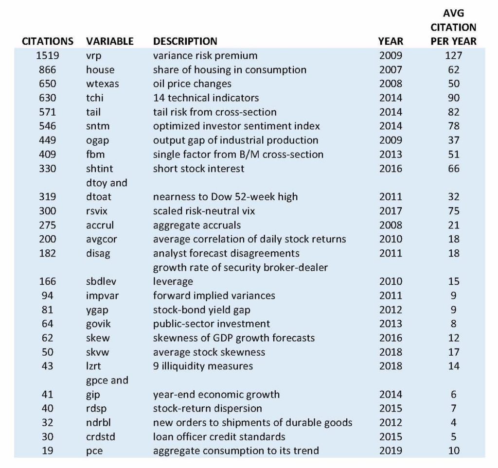
The Five Best Variables on a Statistical Basis

Fourth-Quarter Growth Rate in Personal Consumption Expenditures ( gpce) : This macroeconomic variable from researchers Møller and Rangvid posits that high personal consumption growth rates at the end of the year predicts poor stock-market gains in the following year. The researchers found it to be the best, and most consistent, variable in the investment strategies. It outperformed a buy-and-hold approach with three of the four strategies tested. However, the outperformance was only marginal.

Aggregate Accruals (accru) : This is a sentiment-based variable introduced by Hirshleifer, Hou and Teoh and uses aggressive corporate accounting to predict future stock returns — more aggressive accruals lead to lower future returns. The variable also marginally beat buy-and-hold returns in three out of four approaches. Most of its performance came from its prediction of the post-tech market crash in 2000-2002.

Credit Standards (crdstd) : This is another macroeconomic variable and was introduced by Chava, Gallmeyer and Park. It finds that optimistic (loose) credit standards predict poor market returns and comes from survey data by the Fed. This variable did well in the researchers’ investment strategies and had good performance on test sample data, but statistical measures of the variable on the training sample data were not as convincing and much of its performance comes from the first four years in that sample.

The Investment Capital Ratio (i/k) : This a financial ratio introduced by Cochrane all the way back in 1991 and was also included in the 2008 paper from Goyal and Welch. It posits that high capital investment in the current quarter predicts poor stock-market returns in the next quarter. While it was a poor predictor from 1975 to 1998, it has since improved performance yet was not able to outperform a buy-and-hold strategy in three of four of the researchers’ timing strategies.

Treasury-bill Rates (tbl ): This is another variable examined in the 2008 paper. It does well statistically but had poor performance in the investment strategies.

Oft-Cited Papers With Poor-Performing Variables

Variance Risk Premium (vrp) : This variable was introduced by Bollerslev, Tauchen and Zhou and has the most citations. The variable had poor statistical performance, as well as poor performance in all four of the investment strategies.

Share of Housing Consumption (house) : This macroeconomic variable introduced by Piazzesi, Schneider and Tuzel has the second-highest number of citations. It uses housing share of consumer spending to forecast the excess return of stocks. (The higher the spending on housing, the higher the excess returns in the stock market.) The variable had poor statistical performance on the extended dataset and poor performance in the investment strategies.

The Price of West-Texas Intermediate Crude Oil (wtexas) : This was the only commodity-based variable and was introduced by Driesprong, Jacobsen and Maat. The paper posits that changes in the price of oil predict stock returns — higher oil prices lead to lower stock returns — with lags. The variable had poor statistical performance for the extended dataset and inconsistent performance in the investment strategies.

The First Principal Component of 14 Technical Indicators ( tchi ): This variable was introduced by Neely, Rapach, Tu and Zhou and is a linear combination of technical indicators including moving price averages, momentum and volume. It only had marginal statistical performance and inconsistent performance in the trading strategies.

Featured Faculty

Distinguished Professor of Finance; J. Fred Weston Chair in Finance

About the Research

Goyal, A., Welch, I., & Zafirov, A. (2021). A Comprehensive Look at the Empirical Performance of Equity Premium Prediction II . http://dx.doi.org/10.2139/ssrn.3929119

Suggested Articles

New Study Disavows Marshmallow Test’s Predictive Powers

Replicating a Successful Nudge in Health Care: Advice for Skeptics

Calculating a Value for the Government Support Banks Enjoy

Related articles.

They’re Calling It the AI Bull Market

After launch of ChatGPT, swift reappraisal by investors

Across 145 Years and 17 Countries, a Common Thread in Risky Credit Booms

Do investors misprice assets, revise their risk appetite or make some other misjudgment?

You Call That Fun? Why Individual Stock Investors Bother

Avanidhar Subrahmanyam studies how some investors’ gambling mentality affects share prices

The Strange Case of the Missing Stock Market Return

Investors in leveraged companies take on extra risk, but research indicates they see no offsetting return

Stock Market Trading and Market Conditions

This paper investigates the dynamic relation between market-wide trading activity and returns in 46 markets. Many stock markets exhibit a strong positive relation between turnover and past returns. These findings stand up in the face of various controls for volatility, alternative definitions for turnover, and differing sample periods, and are present at both the weekly and daily frequency. However, the magnitude of this relation varies widely across markets. Several competing explanations are examined by linking cross-country variables to the magnitude of the relation. The relation between returns and turnover is stronger in countries with restrictions on short sales and where stocks are highly cross-correlated; it is also stronger among individual investors than among foreign or institutional investors. In developed economies, turnover follows past returns more strongly in the 1980s than in the 1990s. The evidence is consistent with models of costly stock market participation in which investors infer that their participation is more advantageous following higher stock returns.

• Acknowledgements and Disclosures

MARC RIS BibTeΧ

Download Citation Data

More from NBER

In addition to working papers , the NBER disseminates affiliates’ latest findings through a range of free periodicals — the NBER Reporter , the NBER Digest , the Bulletin on Retirement and Disability , the Bulletin on Health , and the Bulletin on Entrepreneurship  — as well as online conference reports , video lectures , and interviews .

An official website of the United States government

The .gov means it’s official. Federal government websites often end in .gov or .mil. Before sharing sensitive information, make sure you’re on a federal government site.

The site is secure. The https:// ensures that you are connecting to the official website and that any information you provide is encrypted and transmitted securely.

• Publications
• Account settings

Preview improvements coming to the PMC website in October 2024. Learn More or Try it out now .

• Advanced Search
• Journal List
• Entropy (Basel)

Stock Market Volatility and Return Analysis: A Systematic Literature Review

Roni bhowmik.

1 School of Economics and Management, Jiujiang University, Jiujiang 322227, China

2 Department of Business Administration, Daffodil International University, Dhaka 1207, Bangladesh

Shouyang Wang

3 Academy of Mathematics and Systems Science, Chinese Academy of Sciences, Beijing 100080, China; nc.ca.ssma@gnawys

In the field of business research method, a literature review is more relevant than ever. Even though there has been lack of integrity and inflexibility in traditional literature reviews with questions being raised about the quality and trustworthiness of these types of reviews. This research provides a literature review using a systematic database to examine and cross-reference snowballing. In this paper, previous studies featuring a generalized autoregressive conditional heteroskedastic (GARCH) family-based model stock market return and volatility have also been reviewed. The stock market plays a pivotal role in today’s world economic activities, named a “barometer” and “alarm” for economic and financial activities in a country or region. In order to prevent uncertainty and risk in the stock market, it is particularly important to measure effectively the volatility of stock index returns. However, the main purpose of this review is to examine effective GARCH models recommended for performing market returns and volatilities analysis. The secondary purpose of this review study is to conduct a content analysis of return and volatility literature reviews over a period of 12 years (2008–2019) and in 50 different papers. The study found that there has been a significant change in research work within the past 10 years and most of researchers have worked for developing stock markets.

1. Introduction

In the context of economic globalization, especially after the impact of the contemporary international financial crisis, the stock market has experienced unprecedented fluctuations. This volatility increases the uncertainty and risk of the stock market and is detrimental to the normal operation of the stock market. To reduce this uncertainty, it is particularly important to measure accurately the volatility of stock index returns. At the same time, due to the important position of the stock market in the global economy, the beneficial development of the stock market has become the focus. Therefore, the knowledge of theoretical and literature significance of volatility are needed to measure the volatility of stock index returns.

Volatility is a hot issue in economic and financial research. Volatility is one of the most important characteristics of financial markets. It is directly related to market uncertainty and affects the investment behavior of enterprises and individuals. A study of the volatility of financial asset returns is also one of the core issues in modern financial research and this volatility is often described and measured by the variance of the rate of return. However, forecasting perfect market volatility is difficult work and despite the availability of various models and techniques, not all of them work equally for all stock markets. It is for this reason that researchers and financial analysts face such a complexity in market returns and volatilities forecasting.

The traditional econometric model often assumes that the variance is constant, that is, the variance is kept constant at different times. An accurate measurement of the rate of return’s fluctuation is directly related to the correctness of portfolio selection, the effectiveness of risk management, and the rationality of asset pricing. However, with the development of financial theory and the deepening of empirical research, it was found that this assumption is not reasonable. Additionally, the volatility of asset prices is one of the most puzzling phenomena in financial economics. It is a great challenge for investors to get a pure understanding of volatility.

A literature reviews act as a significant part of all kinds of research work. Literature reviews serve as a foundation for knowledge progress, make guidelines for plan and practice, provide grounds of an effect, and, if well guided, have the capacity to create new ideas and directions for a particular area [ 1 ]. Similarly, they carry out as the basis for future research and theory work. This paper conducts a literature review of stock returns and volatility analysis based on generalized autoregressive conditional heteroskedastic (GARCH) family models. Volatility refers to the degree of dispersion of random variables.

Financial market volatility is mainly reflected in the deviation of the expected future value of assets. The possibility, that is, volatility, represents the uncertainty of the future price of an asset. This uncertainty is usually characterized by variance or standard deviation. There are currently two main explanations in the academic world for the relationship between these two: The leverage effect and the volatility feedback hypothesis. Leverage often means that unfavorable news appears, stock price falls, leading to an increase in the leverage factor, and thus the degree of stock volatility increases. Conversely, the degree of volatility weakens; volatility feedback can be simply described as unpredictable stock volatility that will inevitably lead to higher risk in the future.

There are many factors that affect price movements in the stock market. Firstly, there is the impact of monetary policy on the stock market, which is extremely substantial. If a loose monetary policy is implemented in a year, the probability of a stock market index rise will increase. On the other hand, if a relatively tight monetary policy is implemented in a year, the probability of a stock market index decline will increase. Secondly, there is the impact of interest rate liberalization on risk-free interest rates. Looking at the major global capital markets, the change in risk-free interest rates has a greater correlation with the current stock market. In general, when interest rates continue to rise, the risk-free interest rate will rise, and the cost of capital invested in the stock market will rise simultaneously. As a result, the economy is expected to gradually pick up during the release of the reform dividend, and the stock market is expected to achieve a higher return on investment.

Volatility is the tendency for prices to change unexpectedly [ 2 ], however, all kinds of volatility is not bad. At the same time, financial market volatility has also a direct impact on macroeconomic and financial stability. Important economic risk factors are generally highly valued by governments around the world. Therefore, research on the volatility of financial markets has always been the focus of financial economists and financial practitioners. Nowadays, a large part of the literature has studied some characteristics of the stock market, such as the leverage effect of volatility, the short-term memory of volatility, and the GARCH effect, etc., but some researchers show that when adopting short-term memory by the GARCH model, there is usually a confusing phenomenon, as the sampling interval tends to zero. The characterization of the tail of the yield generally assumes an ideal situation, that is, obeys the normal distribution, but this perfect situation is usually not established.

Researchers have proposed different distributed models in order to better describe the thick tail of the daily rate of return. Engle [ 3 ] first proposed an autoregressive conditional heteroscedasticity model (ARCH model) to characterize some possible correlations of the conditional variance of the prediction error. Bollerslev [ 4 ] has been extended it to form a generalized autoregressive conditional heteroskedastic model (GARCH model). Later, the GARCH model rapidly expanded and a GARCH family model was created.

When employing GARCH family models to analyze and forecast return volatility, selection of input variables for forecasting is crucial as the appropriate and essential condition will be given for the method to have a stationary solution and perfect matching [ 5 ]. It has been shown in several findings that the unchanged model can produce suggestively different results when it is consumed with different inputs. Thus, another key purpose of this literature review is to observe studies which use directional prediction accuracy model as a yardstick from a realistic point of understanding and has the core objective of the forecast of financial time series in stock market return. Researchers estimate little forecast error, namely measured as mean absolute deviation (MAD), root mean squared error (RMSE), mean absolute error (MAE), and mean squared error (MSE) which do not essentially interpret into capital gain [ 6 , 7 ]. Some others mention that the predictions are not required to be precise in terms of NMSE (normalized mean squared error) [ 8 ]. It means that finding the low rate of root mean squared error does not feed high returns, in another words, the relationship is not linear between two.

In this manuscript, it is proposed to categorize the studies not only by their model selection standards but also for the inputs used for the return volatility as well as how precise it is spending them in terms of return directions. In this investigation, the authors repute studies which use percentage of success trades benchmark procedures for analyzing the researchers’ proposed models. From this theme, this study’s authentic approach is compared with earlier models in the literature review for input variables used for forecasting volatility and how precise they are in analyzing the direction of the related time series. There are other review studies on return and volatility analysis and GARCH-family based financial forecasting methods done by a number of researchers [ 9 , 10 , 11 , 12 , 13 ]. Consequently, the aim of this manuscript is to put forward the importance of sufficient and necessary conditions for model selection and contribute for the better understanding of academic researchers and financial practitioners.

Systematic reviews have most notable been expanded by medical science as a way to synthesize research recognition in a systematic, transparent, and reproducible process. Despite the opportunity of this technique, its exercise has not been overly widespread in business research, but it is expanding day by day. In this paper, the authors have used the systematic review process because the target of a systematic review is to determine all empirical indication that fits the pre-decided inclusion criteria or standard of response to a certain research question. Researchers proved that GARCH is the most suitable model to use when one has to analysis the volatility of the returns of stocks with big volumes of observations [ 3 , 4 , 6 , 9 , 13 ]. Researchers observe keenly all the selected literature to answer the following research question: What are the effective GARCH models to recommend for performing market volatility and return analysis?

The main contribution of this paper is found in the following four aspects: (1) The best GARCH models can be recommended for stock market returns and volatilities evaluation. (2) The manuscript considers recent papers, 2008 to 2019, which have not been covered in previous studies. (3) In this study, both qualitative and quantitative processes have been used to examine the literature involving stock returns and volatilities. (4) The manuscript provides a study based on journals that will help academics and researchers recognize important journals that they can denote for a literature review, recognize factors motivating analysis stock returns and volatilities, and can publish their worth study manuscripts.

2. Methodology

A systematic literature examination of databases should recognize as complete a list as possible of relevant literature while keeping the number of irrelevant knocks small. The study is conducted by a systematic based literature review, following suggestions from scholars [ 14 , 15 ]. This manuscript was led by a systematic database search, surveyed by cross-reference snowballing, as demonstrated in Figure 1 , which was adapted from Geissdoerfer et al. [ 16 ]. Two databases were selected for the literature search: Scopus and Web-of-Science. These databases were preferred as they have some major depositories of research and are usually used in literature reviews for business research [ 17 ].

Literature review method.

At first stage, a systematic literature search is managed. The keywords that were too broad or likely to be recognized in literature-related keywords with other research areas are specified below. As shown in Table 1 , the search string “market return” in ‘Title‘ respectively “stock market return”, “stock market volatility”, “stock market return volatility”, “GARCH family model* for stock return”, “forecasting stock return”, and GARCH model*, “financial market return and volatility” in ‘Topic’ separately ‘Article title, Abstract, Keywords’ were used to search for reviews of articles in English on the Elsevier Scopus and Thomson Reuters Web-of-Science databases. The asterisk (*) is a commonly used wildcard symbol that broadens a search by finding words that start with the same letters.

Literature search strings for database.

At second stage, suitable cross-references were recognized in this primary sample by first examining the publications’ title in the reference portion and their context and cited content in the text. The abstracts of the recognized further publications were examined to determine whether the paper was appropriate or not. Appropriate references were consequently added to the sample and analogously scanned for appropriate cross-references. This method was continual until no additional appropriate cross-references could be recognized.

At the third stage, the ultimate sample was assimilated, synthesized, and compiled into the literature review presented in the subsequent section. The method was revised a few days before the submission.

Additionally, the list of affiliation criteria in Table 2 , which is formed on discussions of the authors, with the summaries of all research papers were independently checked in a blind system method. Evaluations were established on the content of the abstract, with any extra information unseen, and were comprehensive rather than exclusive. In order to check for inter-coder dependability, an initial sample of 30 abstracts were studied for affiliation by the authors. If the abstract was not satisfactorily enough, the whole paper was studied. Simply, 4.61 percent of the abstract resulted in variance between the researchers. The above-mentioned stages reduced the subsequent number of full papers for examination and synthesis to 50. In order to recognize magnitudes, backgrounds, and moderators, these residual research papers were reviewed in two rounds of reading.

Affiliation criteria.

3. Review of Different Studies

In this paper, a large amount of articles were studied but only a few were well thought out to gather the quality developed earlier. For every published article, three groups were specified. Those groups were considered as index and forecast time period, input elements, econometric models, and study results. The first group namely “index and forecast time period with input elements” was considered since market situation like emerging, frontier, and developed markets which are important parameters of forecast and also the length of evaluation is a necessary characteristic for examining the robustness of the model. Furthermore, input elements are comparatively essential parameters for a forecast model because the analytical and diagnostic ability of the model is mainly supported on the inputs that a variable uses. In the second group, “model” was considered forecast models proposed by authors and other models for assessment. The last group is important to our examination for comparing studies in relationships of proper guiding return and volatility, acquired by using recommended estimate models, named the “study results” group.

Measuring the stock market volatility is an incredibly complex job for researchers. Since volatility tends to cluster, if today’s volatility is high, it is likely to be high tomorrow but they have also had an attractive high hit rate with major disasters [ 4 , 7 , 11 , 12 ]. GARCH models have a strong background, recently having crossed 30 years of the fast progress of GARCH-type models for investigating the volatility of market data. Literature of eligible papers were clustered in two sub groups, the first group containing GARCH and its variations model, and the second group containing bivariate and other multivariate GARCH models, summarized in a table format for future studies. Table 3 explains the review of GARCH and its variations models. The univariate GARCH model is for a single time series. It is a statistical model that is used to analyze a number of different kinds of financial data. Financial institutions and researchers usually use this model to estimate the volatility of returns for stocks, bonds, and market indices. In the GARCH model, current volatility is influenced by past innovation to volatility. GARCH models are used to model for forecast volatility of one time series. The most widely used GARCH form is GARCH (1, 1) and this has some extensions.

Different literature studies based on generalized autoregressive conditional heteroskedastic (GARCH) and its variations models.

Notes: APARCH (Asymmetric Power ARCH), AIC (Akaike Information Criterion), OHLC (Open-High-Low-Close Chart), NSE (National Stock Exchange of India), EWMA (Exponentially Weighted Moving Average), CGARCH (Component GARCH), BDS (Brock, Dechert & Scheinkman) Test, ARCH-LM (ARCH-Lagrange Multiplier) test, VAR (Vector Autoregression) model, VEC (Vector Error Correction) model, ARFIMA (Autoregressive Fractional Integral Moving Average), FIGARCH (Fractionally Integrated GARCH), SHCI (Shanghai Stock Exchange Composite Index), SZCI (Shenzhen Stock Exchange Component Index), ADF (Augmented Dickey–Fuller) test, BSE (Bombay Stock Exchange), and PGARCH (Periodic GARCH) are discussed.

In a simple GARCH model, the squared volatility σ t 2 is allowed to change on previous squared volatilities, as well as previous squared values of the process. The conditional variance satisfies the following form: σ t 2 = α 0 + α 1 ϵ t − 1 2 + … + α q ϵ t − q 2 + β 1 σ t − 1 2 + … + β p σ t − p 2 where, α i > 0 and β i > 0 . For the GARCH model, residuals’ lags can substitute by a limited number of lags of conditional variances, which abridges the lag structure and in addition the estimation method of coefficients. The most often used GARCH model is the GARCH (1, 1) model. The GARCH (1, 1) process is a covariance-stationary white noise process if and only if α 1 + β < 1 . The variance of the covariance-stationary process is given by α 1   /   ( 1 − α 1 − β ) . It specifies that σ n 2     is based on the most recent observation of φ t 2   and the most recent variance rate σ n − 1 2 . The GARCH (1, 1) model can be written as σ n 2 = ω + α φ n − 1 2 + β σ n − 1 2 and this is usually used for the estimation of parameters in the univariate case.

Though, GARCH model is not a complete model, and thus could be developed, these developments are detected in the form of the alphabet soup that uses GARCH as its key component. There are various additions of the standard GARCH family models. Nonlinear GARCH (NGARCH) was proposed by Engle and Ng [ 18 ]. The conditional covariance equation is in the form: σ t 2 = γ + α ( ε t − 1 − ϑ σ t − 1   ) 2 + β σ t − 1 2 , where α ,   β ,   γ > 0 . The integrated GARCH (IGARCH) is a restricted version of the GARCH model, where the sum of all the parameters sum up to one and this model was introduced by Engle and Bollerslev [ 19 ]. Its phenomenon might be caused by random level shifts in volatility. The simple GARCH model fails in describing the “leverage effects” which are detected in the financial time series data. The exponential GARCH (EGARCH) introduced by Nelson [ 5 ] is to model the logarithm of the variance rather than the level and this model accounts for an asymmetric response to a shock. The GARCH-in-mean (GARCH-M) model adds a heteroskedasticity term into the mean equation and was introduced by Engle et al. [ 20 ]. The quadratic GARCH (QGARCH) model can handle asymmetric effects of positive and negative shocks and this model was introduced by Sentana [ 21 ]. The Glosten-Jagannathan-Runkle GARCH (GJR-GARCH) model was introduced by Glosten et al. [ 22 ], its opposite effects of negative and positive shocks taking into account the leverage fact. The threshold GARCH (TGARCH) model was introduced by Zakoian [ 23 ], this model is also commonly used to handle leverage effects of good news and bad news on volatility. The family GARCH (FGARCH) model was introduced by Hentschel [ 24 ] and is an omnibus model that is a mix of other symmetric or asymmetric GARCH models. The COGARCH model was introduced by Klüppelberg et al. [ 25 ] and is actually the stochastic volatility model, being an extension of the GARCH time series concept to continuous time. The power-transformed and threshold GARCH (PTTGARCH) model was introduced by Pan et al. [ 26 ], this model is a very flexible model and, under certain conditions, includes several ARCH/GARCH models.

Based on the researchers’ articles, the symmetric GARCH (1, 1) model has been used widely to forecast the unconditional volatility in the stock market and time series data, and has been able to simulate the asset yield structure and implied volatility structure. Most researchers show that GARCH (1, 1) with a generalized distribution of residual has more advantages in volatility assessment than other models. Conversely, the asymmetry influence in stock market volatility and return analysis was beyond the descriptive power of the asymmetric GARCH models, as the models could capture more specifics. Besides, the asymmetric GARCH models can incompletely measure the effect of positive or negative shocks in stock market return and volatility, and the GARCH (1, 1) comparatively failed to accomplish this fact. In asymmetric effect, the GJR-GARCH model performed better and produced a higher predictable conditional variance during the period of high volatility. In addition, among the asymmetric GARCH models, the reflection of EGARCH model appeared to be superior.

Table 4 has explained the review of bivariate and other multivariate GARCH models. Bivariate model analysis was used to find out if there is a relationship between two different variables. Bivariate model uses one dependent variable and one independent variable. Additionally, the Multivariate GARCH model is a model for two or more time series. Multivariate GARCH models are used to model for forecast volatility of several time series when there are some linkages between them. Multivariate model uses one dependent variable and more than one independent variable. In this case, the current volatility of one time series is influenced not only by its own past innovation, but also by past innovations to volatilities of other time series.

Different literature studies based on bivariate and other multivariate GARCH models.

The most recognizable use of multivariate GARCH models is the analysis of the relations between the volatilities and co-volatilities of several markets. A multivariate model would create a more dependable model than separate univariate models. The vector error correction (VEC) models is the first MGARCH model which was introduced by Bollerslev et al. [ 66 ]. This model is typically related to subsequent formulations. The model can be expressed in the following form: v e c h   ( H t ) = ℂ + ∑ j = 1 q X j   v e c h   ( ϵ t − j   ϵ t − j ' ) + ∑ j = 1 p Y j   v e c h   ( H t − j   )   where v e c h is an operator that stacks the columns of the lower triangular part of its argument square matrix and H t is the covariance matrix of the residuals. The regulated version of the VEC model is the DVEC model and was also recommended by Bollerslev et al. [ 66 ]. Compared to the VEC model, the estimation method proceeded far more smoothly in the DVEC model. The Baba-Engle-Kraft-Kroner (BEKK) model was introduced by Baba et al. [ 67 ] and is an innovative parameterization of the conditional variance matrix H t . The BEKK model accomplishes the positive assurance of the conditional covariance by conveying the model in a way that this property is implied by the model structure. The Constant Conditional Correlation (CCC) model was recommended by Bollerslev [ 68 ], to primarily model the conditional covariance matrix circuitously by estimating the conditional correlation matrix. The Dynamic Conditional Correlation (DCC) model was introduced by Engle [ 69 ] and is a nonlinear mixture of univariate GARCH models and also a generalized variety of the CCC model. To overcome the inconveniency of huge number of parameters, the O-GARCH model was recommended by Alexander and Chibumba [ 70 ] and consequently developed by Alexander [ 71 , 72 ]. Furthermore, a multivariate GARCH model GO-GARCH model was introduced by Bauwens et al. [ 73 ].

The bivariate models showed achieve better in most cases, compared with the univariate models [ 85 ]. MGARCH models could be used for forecasting. Multivariate GARCH modeling delivered a realistic but parsimonious measurement of the variance matrix, confirming its positivity. However, by analyzing the relative forecasting accuracy of the two formulations, BEKK and DCC, it could be deduced that the forecasting performance of the MGARCH models was not always satisfactory. By comparing it with the other multivariate GARCH models, BEKK-GARCH model was comparatively better and flexible but it needed too many parameters for multiple time series. Conversely, for the area of forecasting, the DCC-GARCH model was more parsimonious. In this regard, it was significantly essential to balance parsimony and flexibility when modeling multivariate GARCH models.

The current systematic review has identified 50 research articles for studies on significant aspects of stock market return and volatility, review types, and GARCH model analysis. This paper noticed that all the studies in this review used an investigational research method. A literature review is necessary for scholars, academics, and practitioners. However, assessing various kinds of literature reviews can be challenging. There is no use for outstanding and demanding literature review articles, since if they do not provide a sufficient contribution and something that is recent, it will not be published. Too often, literature reviews are fairly descriptive overviews of research carried out among particular years that draw data on the number of articles published, subject matter covered, authors represented, and maybe methods used, without conducting a deeper investigation. However, conducting a literature review and examining its standard can be challenging, for this reason, this article provides some rigorous literature reviews and, in the long run, to provide better research.

4. Conclusions

Working on a literature review is a challenge. This paper presents a comprehensive literature which has mainly focused on studies on return and volatility of stock market using systematic review methods on various financial markets around the world. This review was driven by researchers’ available recommendations for accompanying systematic literature reviews to search, examine, and categorize all existing and accessible literature on market volatility and returns [ 16 ]. Out of the 435 initial research articles located in renowned electronic databases, 50 appropriate research articles were extracted through cross-reference snowballing. These research articles were evaluated for the quality of proof they produced and were further examined. The raw data were offered by the authors from the literature together with explanations of the data and key fundamental concepts. The outcomes, in this research, delivered future magnitudes to research experts for further work on the return and volatility of stock market.

Stock market return and volatility analysis is a relatively important and emerging field of research. There has been plenty of research on financial market volatility and return because of easily increasing accessibility and availability of researchable data and computing capability. The GARCH type models have a good model on stock market volatilities and returns investigation. The popularity of various GARCH family models has increased in recent times. Every model has its specific strengths and weaknesses and has at influence such a large number of GARCH models. To sum up the reviewed papers, many scholars suggest that the GARCH family model provides better results combined with another statistical technique. Based on the study, much of the research showed that with symmetric information, GARCH (1, 1) could precisely explain the volatilities and returns of the data and when under conditions of asymmetric information, the asymmetric GARCH models would be more appropriate [ 7 , 32 , 40 , 47 , 48 ]. Additionally, few researchers have used multivariate GARCH model statistical techniques for analyzing market volatility and returns to show that a more accurate and better results can be found by multivariate GARCH family models. Asymmetric GARCH models, for instance and like, EGARCH, GJR GARCH, and TGARCH, etc. have been introduced to capture the effect of bad news on the change in volatility of stock returns [ 42 , 58 , 62 ]. This study, although short and particular, attempted to give the scholar a concept of different methods found in this systematic literature review.

With respect to assessing scholars’ articles, the finding was that rankings and specifically only one GARCH model was sensitive to the different stock market volatilities and returns analysis, because the stock market does not have similar characteristics. For this reason, the stock market and model choice are little bit difficult and display little sensitivity to the ranking criterion and estimation methodology, additionally applying software is also another matter. The key challenge for researchers is finding the characteristics in stock market summarization using different kinds of local stock market returns, volatility detection, world stock market volatility, returns, and other data. Additional challenges are modeled by differences of expression between different languages. From an investigation perception, it has been detected that different authors and researchers use special datasets for the valuation of their methods, which may put boundary assessments between research papers.

Whenever there is assurance that scholars build on high accuracy, it will be easier to recognize genuine research gaps instead of merely conducting the same research again and again, so as to progress better and create more appropriate hypotheses and research questions, and, consequently, to raise the standard of research for future generation. This study will be beneficial for researchers, scholars, stock exchanges, regulators, governments, investors, and other concerned parties. The current study also contributes to the scope of further research in the area of stock volatility and returns. The content analysis can be executed taking the literature of the last few decades. It determined that a lot of methodologies like GARCH models, Johansen models, VECM, Impulse response functions, and Granger causality tests are practiced broadly in examining stock market volatility and return analysis across countries as well as among sectors with in a country.

Author Contributions

R.B. and S.W. proposed the research framework together. R.B. collected the data, and wrote the document. S.W. provided important guidance and advice during the process of this research. All authors have read and agreed to the published version of the manuscript.

This research received no external funding.

Conflicts of Interest

The authors declare no conflict of interest.

• Number of Visitor : 9542048

• About Research
• Advisory Committee
• Research Paper/ Articles
• Upcoming Conferences

• Certifications
• NISM Newsletters
• Investor Education

China Drafts Rules on Tighter Stock Trading, Listing Regulations

FILE PHOTO: A Chinese national flag flutters outside the China Securities Regulatory Commission (CSRC) building on the Financial Street in Beijing, China July 9, 2021. REUTERS/Tingshu Wang/File Photo

SHANGHAI (Reuters) -China's securities regulator issued draft rules on Friday to strengthen the supervision of company listings, delistings and computer-driven programme trading, in a move to improve the stock market and protect investors' interests.

The China Securities Regulatory Commission (CSRC) will raise the bar for initial public offerings (IPOs), force unqualified companies to delist, and strengthen the oversight of high-frequency trading, according to draft rules put out for public opinion.

Chinese authorities are stepping up efforts to revive investor confidence in the world's second-biggest stock market. The blue-chip index has rebounded from five-year lows hit in February but is still struggling to stand on its feet.

"We will orient toward value centred around people and protect investors, especially small investors, more effectively," CSRC Chairman Wu Qing said in an article posted on the watchdog's website.

"We will set up a comprehensive supervision system so as to regulate with 'teeth and thorns'", said Wu, who earned the nickname "broker butcher" during a previous regulatory stint.

To improve the quality of listed companies, the CSRC said it plans to moderately increase the listing requirements in terms of sales and net profit for companies seeking to float on the main board and tech-focused ChiNext.

The bar will also be raised for companies targeting Shanghai's tech-focused STAR Market.

Meanwhile, regulators will boost the number of randomly selected onsite inspections to 20% of listing candidates, from 5% previously. The number of onsite inspections on underwriters will also be increased, the CSRC said.

PROGRAMME TRADING

The CSRC also proposed tighter scrutiny of programme trading and high-frequency trading to maintain market fairness.

The regulator already cracked down on data-driven quant funds early this year, saying some institutions command unfair advantage over retail investors. In February, Chinese bourses barred a quant fund manager from trading for three days, saying it had broken rules on orderly trading.

Programme trading, in which orders are automatically placed using computers, "must abide by the principle of fairness, and must not endanger the exchange system, or disturb market order," CSRC said in draft rules on Friday.

The rules call for setting up a reporting system for programme trading, with high-frequency trading subject to higher disclosure requirements and higher fees.

Both domestic and foreign capital will be included in the transaction reporting system and be subject to the same transaction monitoring standards, the CSRC added.

(Reporting by Shanghai and Beijing Newsrooms; Editing by David Goodman, Susan Fenton and Hugh Lawson)

Copyright 2024 Thomson Reuters .

Tags: funds , Asia , financial regulation

The Best Financial Tools for You

Credit Cards

Personal Loans

Comparative assessments and other editorial opinions are those of U.S. News and have not been previously reviewed, approved or endorsed by any other entities, such as banks, credit card issuers or travel companies. The content on this page is accurate as of the posting date; however, some of our partner offers may have expired.

Subscribe to our daily newsletter to get investing advice, rankings and stock market news.

See a newsletter example .

You May Also Like

10 best value stocks to buy now.

Ian Bezek April 12, 2024

Water Stocks and ETFs

Matt Whittaker April 12, 2024

7 Stocks Jeff Bezos Is Buying

Jeff Reeves April 12, 2024

Is It Time to Invest Internationally?

Kate Stalter April 11, 2024

Cheap Dividend Stocks to Buy Under $10

Wayne Duggan April 11, 2024

5 Best Large-Cap Growth Stocks

Glenn Fydenkevez April 11, 2024

7 Dividend Kings to Buy and Hold Forever

Tony Dong April 11, 2024

5 Socially Responsible Investing Apps

Coryanne Hicks April 10, 2024

7 Diabetes and Weight Loss Drug Stocks

Brian O'Connell April 10, 2024

7 Best Socially Responsible Funds

Jeff Reeves April 10, 2024

Fidelity Mutual Funds to Buy and Hold

Tony Dong April 10, 2024

Dividend Stocks to Buy and Hold

Wayne Duggan April 9, 2024

What Is a Stock Market Correction?

Marc Guberti April 9, 2024

If You Invested $10,000 in SMCI IPO

6 of the Best AI ETFs to Buy Now

Tony Dong April 9, 2024

7 Best Cybersecurity Stocks to Buy

Glenn Fydenkevez April 8, 2024

How Bitcoin Mining Is Evolving 

Matt Whittaker April 8, 2024

9 of the Best Bond ETFs to Buy Now

Tony Dong April 8, 2024

10 Best Tech Stocks to Buy for 2024

Wayne Duggan April 8, 2024

About the Methodology

U.S. News Staff April 8, 2024

We use cookies to understand how you use our site and to improve your experience. This includes personalizing content and advertising. To learn more, click here . By continuing to use our site, you accept our use of cookies, revised Privacy Policy and Terms of Service .

New to Zacks? Get started here.

Member Sign In

Don't Know Your Password?

• Zacks #1 Rank
• Zacks Industry Rank
• Zacks Sector Rank
• Equity Research
• Mutual Funds
• Mutual Fund Screener
• ETF Screener
• Earnings Calendar
• Earnings Releases
• Earnings ESP
• Earnings ESP Filter
• Stock Screener
• Premium Screens
• Basic Screens
• Research Wizard
• Personal Finance
• Money Managing
• Real Estate
• Retirement Planning
• Tax Information
• My Portfolio
• Create Portfolio
• Style Scores
• Testimonials
• Zacks.com Tutorial

Services Overview

• Zacks Ultimate
• Zacks Investor Collection
• Zacks Premium

Investor Services

• ETF Investor
• Home Run Investor
• Income Investor
• Stocks Under $10
• Value Investor
• Top 10 Stocks

Other Services

• Method for Trading
• Zacks Confidential

Trading Services

• Black Box Trader
• Counterstrike
• Headline Trader
• Insider Trader
• Large-Cap Trader
• Options Trader
• Short Sell List
• Surprise Trader
• Alternative Energy

You are being directed to ZacksTrade, a division of LBMZ Securities and licensed broker-dealer. ZacksTrade and Zacks.com are separate companies. The web link between the two companies is not a solicitation or offer to invest in a particular security or type of security. ZacksTrade does not endorse or adopt any particular investment strategy, any analyst opinion/rating/report or any approach to evaluating individual securities.

If you wish to go to ZacksTrade, click OK . If you do not, click Cancel.

Image: Bigstock

Caterpillar (CAT) Stock Declines While Market Improves: Some Information for Investors

Caterpillar ( CAT Quick Quote CAT - Free Report ) closed the most recent trading day at $371.98, moving -0.02% from the previous trading session. The stock's change was less than the S&P 500's daily gain of 0.74%. Elsewhere, the Dow lost 0.01%, while the tech-heavy Nasdaq added 1.68%.

The construction equipment company's stock has climbed by 8.95% in the past month, exceeding the Industrial Products sector's gain of 3.51% and the S&P 500's gain of 0.8%.

The investment community will be paying close attention to the earnings performance of Caterpillar in its upcoming release. In that report, analysts expect Caterpillar to post earnings of $5.11 per share. This would mark year-over-year growth of 4.07%. Our most recent consensus estimate is calling for quarterly revenue of $15.99 billion, up 0.78% from the year-ago period.

For the full year, the Zacks Consensus Estimates project earnings of $21.33 per share and a revenue of $67.61 billion, demonstrating changes of +0.57% and +0.82%, respectively, from the preceding year.

It's also important for investors to be aware of any recent modifications to analyst estimates for Caterpillar. These latest adjustments often mirror the shifting dynamics of short-term business patterns. Consequently, upward revisions in estimates express analysts' positivity towards the company's business operations and its ability to generate profits.

Our research suggests that these changes in estimates have a direct relationship with upcoming stock price performance. To utilize this, we have created the Zacks Rank, a proprietary model that integrates these estimate changes and provides a functional rating system.

The Zacks Rank system, running from #1 (Strong Buy) to #5 (Strong Sell), holds an admirable track record of superior performance, independently audited, with #1 stocks contributing an average annual return of +25% since 1988. Over the last 30 days, the Zacks Consensus EPS estimate has witnessed a 0.49% increase. Caterpillar is currently sporting a Zacks Rank of #2 (Buy).

Looking at its valuation, Caterpillar is holding a Forward P/E ratio of 17.44. This signifies a premium in comparison to the average Forward P/E of 10.77 for its industry.

We can also see that CAT currently has a PEG ratio of 1.66. This metric is used similarly to the famous P/E ratio, but the PEG ratio also takes into account the stock's expected earnings growth rate. The Manufacturing - Construction and Mining industry currently had an average PEG ratio of 1.04 as of yesterday's close.

The Manufacturing - Construction and Mining industry is part of the Industrial Products sector. This industry, currently bearing a Zacks Industry Rank of 69, finds itself in the top 28% echelons of all 250+ industries.

The Zacks Industry Rank evaluates the power of our distinct industry groups by determining the average Zacks Rank of the individual stocks forming the groups. Our research shows that the top 50% rated industries outperform the bottom half by a factor of 2 to 1.

Keep in mind to rely on Zacks.com to watch all these stock-impacting metrics, and more, in the succeeding trading sessions.

See More Zacks Research for These Tickers

Normally $25 each - click below to receive one report free:.

Caterpillar Inc. (CAT) - free report >>

Published in

This file is used for Yahoo remarketing pixel add

Due to inactivity, you will be signed out in approximately: