the flood case study solution

• 0 Shopping Cart

Kerala flood case study

Kerala flood case study.

Kerala is a state on the southwestern Malabar Coast of India. The state has the 13th largest population in India. Kerala, which lies in the tropical region, is mainly subject to the humid tropical wet climate experienced by most of Earth’s rainforests.

A map to show the location of Kerala

Eastern Kerala consists of land infringed upon by the Western Ghats (western mountain range); the region includes high mountains, gorges, and deep-cut valleys. The wildest lands are covered with dense forests, while other areas lie under tea and coffee plantations or other forms of cultivation.

The Indian state of Kerala receives some of India’s highest rainfall during the monsoon season. However, in 2018 the state experienced its highest level of monsoon rainfall in decades. According to the India Meteorological Department (IMD), there was 2346.3 mm of precipitation, instead of the average 1649.55 mm.

Kerala received over two and a half times more rainfall than August’s average. Between August 1 and 19, the state received 758.6 mm of precipitation, compared to the average of 287.6 mm, or 164% more. This was 42% more than during the entire monsoon season.

The unprecedented rainfall was caused by a spell of low pressure over the region. As a result, there was a perfect confluence of the south-west monsoon wind system and the two low-pressure systems formed over the Bay of Bengal and Odisha. The low-pressure regions pull in the moist south-west monsoon winds, increasing their speed, as they then hit the Western Ghats, travel skywards, and form rain-bearing clouds.

Further downpours on already saturated land led to more surface run-off causing landslides and widespread flooding.

Kerala has 41 rivers flowing into the Arabian Sea, and 80 of its dams were opened after being overwhelmed. As a result, water treatment plants were submerged, and motors were damaged.

In some areas, floodwater was between 3-4.5m deep. Floods in the southern Indian state of Kerala have killed more than 410 people since June 2018 in what local officials said was the worst flooding in 100 years. Many of those who died had been crushed under debris caused by landslides. More than 1 million people were left homeless in the 3,200 emergency relief camps set up in the area.

Parts of Kerala’s commercial capital, Cochin, were underwater, snarling up roads and leaving railways across the state impassable. In addition, the state’s airport, which domestic and overseas tourists use, was closed, causing significant disruption.

Local plantations were inundated by water, endangering the local rubber, tea, coffee and spice industries.

Schools in all 14 districts of Kerala were closed, and some districts have banned tourists because of safety concerns.

Maintaining sanitation and preventing disease in relief camps housing more than 800,000 people was a significant challenge. Authorities also had to restore regular clean drinking water and electricity supplies to the state’s 33 million residents.

Officials have estimated more than 83,000km of roads will need to be repaired and that the total recovery cost will be between £2.2bn and $2.7bn.

Indians from different parts of the country used social media to help people stranded in the flood-hit southern state of Kerala. Hundreds took to social media platforms to coordinate search, rescue and food distribution efforts and reach out to people who needed help. Social media was also used to support fundraising for those affected by the flooding. Several Bollywood stars supported this.

Some Indians have opened up their homes for people from Kerala who were stranded in other cities because of the floods.

Thousands of troops were deployed to rescue those caught up in the flooding. Army, navy and air force personnel were deployed to help those stranded in remote and hilly areas. Dozens of helicopters dropped tonnes of food, medicine and water over areas cut off by damaged roads and bridges. Helicopters were also involved in airlifting people marooned by the flooding to safety.

More than 300 boats were involved in rescue attempts. The state government said each boat would get 3,000 rupees (£34) for each day of their work and that authorities would pay for any damage to the vessels.

As the monsoon rains began to ease, efforts increased to get relief supplies to isolated areas along with clean up operations where water levels were falling.

Millions of dollars in donations have poured into Kerala from the rest of India and abroad in recent days. Other state governments have promised more than $50m, while ministers and company chiefs have publicly vowed to give a month’s salary.

Even supreme court judges have donated $360 each, while the British-based Sikh group Khalsa Aid International has set up its own relief camp in Kochi, Kerala’s main city, to provide meals for 3,000 people a day.

International Response

In the wake of the disaster, the UAE, Qatar and the Maldives came forward with offers of financial aid amounting to nearly £82m. The United Arab Emirates promised $100m (£77m) of this aid. This is because of the close relationship between Kerala and the UAE. There are a large number of migrants from Kerala working in the UAE. The amount was more than the $97m promised by India’s central government. However, as it has done since 2004, India declined to accept aid donations. The main reason for this is to protect its image as a newly industrialised country; it does not need to rely on other countries for financial help.

Google provided a donation platform to allow donors to make donations securely. Google partners with the Center for Disaster Philanthropy (CDP), an intermediary organisation that specialises in distributing your donations to local nonprofits that work in the affected region to ensure funds reach those who need them the most.

Google Kerala Donate

Tales of humanity and hope

Check your understanding.

Premium Resources

Please support internet geography.

If you've found the resources on this page useful please consider making a secure donation via PayPal to support the development of the site. The site is self-funded and your support is really appreciated.

Related Topics

Use the images below to explore related GeoTopics.

River flooding and management

Topic home, wainfleet floods case study, share this:.

• Click to share on Twitter (Opens in new window)
• Click to share on Facebook (Opens in new window)
• Click to share on Pinterest (Opens in new window)
• Click to email a link to a friend (Opens in new window)
• Click to share on WhatsApp (Opens in new window)
• Click to print (Opens in new window)

If you've found the resources on this site useful please consider making a secure donation via PayPal to support the development of the site. The site is self-funded and your support is really appreciated.

Search Internet Geography

Top posts and pages.

Latest Blog Entries

Pin It on Pinterest

• Click to share
• Print Friendly

Thank you for visiting nature.com. You are using a browser version with limited support for CSS. To obtain the best experience, we recommend you use a more up to date browser (or turn off compatibility mode in Internet Explorer). In the meantime, to ensure continued support, we are displaying the site without styles and JavaScript.

• View all journals
• My Account Login
• Explore content
• About the journal
• Publish with us
• Sign up for alerts
• Open access
• Published: 25 April 2023

Developing assessment flow for damage estimation of mud housing typology through a case study against coastal floods

• N. Aishwarya 1 ,
• K. Aniruddha 1 ,
• D. Sutapa 2 &
• H. A. Bharath 1  

Scientific Reports volume  13 , Article number:  6712 ( 2023 ) Cite this article

1060 Accesses

2 Citations

Metrics details

• Natural hazards
• Sustainability

Rising instances of prolonged inundation due to climate-aggravated high tide flooding are economically burdensome for resource-crunched developing nations that bear enormous damage due to loss of built infrastructure (housing in this case). Regardless of the loss, coastal flood impact on buildings is rarely given precedence. The mud building typology in India captures 34% of existing housing demand primarily within ruralIndia; for instance, 75% of the housing in Sagar Island uses mud as the dominant construction material, making it an ideal case for the proposed research. The multivariate nature of damage and empirical data constraint associated with mud buildings propels the development of two unconventional damage assessment approaches using multivariate-probabilistic technique. The proposed literature-based approach uses logical reasoning based on the available scientific evidence whereas the lab-based approach uses the insights from structural analysis of scaled model. The damage matrix created from both the approaches are used to analyse a common flood data (depth & duration) generated using 1000 Montecarlo simulations. The resultant Damage Stage values confirm the versatility of either approach over spatial (local to regional)—temporal (flood character and intensity) dimensions. The lab-based approach proved to be a better alternative considering the availability of continuous records on damage behaviour and precise information on the flood threshold of dominant building material, a crucial component of the multivariate damage assessment process.

Similar content being viewed by others

Deriving expert-driven seismic and wind fragility functions for non-engineered residential typologies in Batanes, Philippines

Arvin Hadlos, Aaron Opdyke & S. Ali Hadigheh

GIS-based hydrodynamic modeling for urban flood mitigation in fast-growing regions: a case study of Erbil, Kurdistan Region of Iraq

Andam Mustafa, Michał Szydłowski, … Hasan Mohammed Hameed

Urban growth modelling and social vulnerability assessment for a hazardous Kathmandu Valley

Carlos Mesta, Gemma Cremen & Carmine Galasso

Introduction

Coastal flooding due to high tide anomalies is calamitous, precisely due to prolonged inundation causing widespread destruction of livelihood, housing, and infrastructure in low-lying coastal areas 1 , 2 , 3 , 4 , 5 . The anomalies in this paper refers to the tidal water height that causes prolonged flooding within the low-lying coastal areas 6 . The spatial (geographical extent) and temporal (annual frequency) intensity of such high tides flooding are likely to enhance in the rapidly changing climate scenario that leads to an unprecedented rise in the mean sea level (MSL) 7 , 8 . South East Asia is among the major victims of MSL rise as it exposes around 300 million people (93 million in China, 42 million in Bangladesh, and 36 million in India) to potential risk of coastal flooding 9 , 10 . About 60 percent of this population located in low-elevation coastal zones of South Asia is rural and underequipped to invest in climate-resilient infrastructure 11 . Hence, the recurring floods would be economically burdensome for resource-crunched developing countries 12 , 13 , 14 , 15 , 16 .

India lost about 4.6 million US$ due to floods between 1953 and 2016, including the value of 1.2 million fully and partially damaged housing. The state of West Bengal accounts for 40% of the total housing loss 17 . The housing damage during cyclone Bulbul (2019), Aamphan (2020), and Yaas (2021) was approximated between 0.28 million, 2.86 million to 0.3 million houses in the affected district of West Bengal 18 , 19 . The loss of housing is critical as it affects mental, social, and economic well-being, inflicting chronic poverty and large-scale climate-induced displacements 20 , 21 , 22 , 23 , 24 . Regardless of the loss, coastal flood impact on buildings is rarely given precedence in developing countries due to its resource-intensive character, absence of aboriginal damage catalogues/damage records, and discreet behaviour based on building typology, preventing adaption of the foreign damage curves on native buildings.

For instance, little is known about the flood damage behaviour associated with mud housing. Mud buildings have displayed global dominance as vernacular construction style, fulfilling the housing requirements, particularly within developing countries, because of the climate benefits and associated affordability 25 , 26 , 27 . In India, mud housing, also referred to as non-engineered or kutcha housing, comprising about 34% of the total housing stock (Ministry of Housing and Urban Poverty Alleviation 28 , 29 , 30 , if integrated with disaster-resilient techniques, can relinquish the shortage of 18.78 million housing among the low-income groups 31 , 32 . Hence, investigation regarding the prevailing cost of damage is critical for investing in flood resilient housing schemes as it requires economic appraisals for optimal resource distribution within developing nations 33 .

Damage behaviour in the case of mud buildings

In mud buildings, the damage behaviour depends on ‘prolonged inundation’ along with flood depth as a prominent reason for failure 28 , 34 , 35 . The convenience of interpreting depth values through visual inspections and measuring gauges in the post-hazard scenario has popularized its conduct over other flood characteristics in an empirical data analysis/processing 36 , 37 , 38 , 39 , 40 . Islam 41 was the first to consider a multivariate approach for mud housings using depth and duration variables. The data used was synthetic, and the study clearly stated that the deterministic approach was inconsistent (actual damage data) in portraying the relationship between depth and duration variables.

Multivariate probabilistic damage models can handle this inconsistency reasonably well with their ability to integrate multiple flood characters and data variance in the estimation process 39 . Unlike empirical, the synthetically manifested data using the probabilistic model can be extrapolated over spatial (local to regional) and temporal dimensions (flood character and intensity), allowing pragmatic application in the data-scarce region 42 , 43 . However, estimation, calibration, and validation of the probable loss in response to the synthetic damage data require reliable knowledge of the mud housing damage behaviour(fragility function or curve). Its absence which is also referred to as predefined Damage Stages (DS) in the case of mud housing, limits the ability of the research community and local authorities to estimate the total cost of flood damage. The predefined damage curves suggest the probable loss in response to ‘the degree of physical damage’ incurred when the building is in direct contact with floodwater. It is represented on a scale of 0 (no loss) to 1 (total loss) on the Y-axis with respective flood intensity on X-axis. The loss is correlated to the monetary liabilities required to repair or reconstruct building components. The damage matrix is not to be confused with damage curves in this paper as it discusses the behavioural aspect of one (particular) building that can generically define the damage behaviour of its entire typology in the absence of observed data 44 , 45 , 46 , 47 . Therefore, this research aims to propose two distinct approaches (literature and lab-based approach) based on multivariate-probabilistic technique for evaluating the mud building damage behaviour, applicable in data-scarce region.

The model proposed uses the ‘wattle and daub’ construction technique for its depiction. It is a dominant housing typology practiced among the densely populated rural settlements in the coastal district of West Bengal, India. The coastal Bengal belongs to the habited part of the largest mangrove forest Sundarbans—the United Nations Educational, Scientific and Cultural Organization (UNESCO) heritage site cleared in the early 1800s for cultivation. The region is highly vulnerable to slow-rising coastal floods, which have become more common in the past ten years. Figure  1 presents a glimpse of the post-flood situation of affected regions, primarily Sagar Island. The Island, with an area of about 282 sq. km (in Fig.  2 ) is located between 21.6276° N to 21.8842° N and 88.0408° E to 88.1278° E in South 24 Paraganas, and has witnessed repeated incidents of high tidal anomalies 48 , 49 . The most pronounced flood incidents were recorded during cyclone Aila (2009) and the last three consecutive cyclones, Bulbul (2019), Aamphan (2020), and Yaas (2021). The Island saw an exponential growth of 37% from 1991 (0.15 million) to 2011 (0.21 million), with a severely marginalized population due to the prevalence of extreme poverty, isolation from the mainland, and lack of organized support. The government compensation for post-flood housing restoration is insufficient to put forward the idea of 'building back better' (BBB) that is undoubtedly a priority for proactive adaptation to climate change.

Inundation, post inundation scenario along with primary housing typology at Sagar.

Study area—Sagar Island (West Bengal, India).

The paper estimates the damage behaviour of mud buildings based on a multivariate probabilistic technique using two pragmatic approaches as described in Fig.  3 , (a) literature-based and (b) laboratory-based approach 50 , 51 . In the literature-based approach, the damage behaviour of mud building is marked using logical assumptions from the available scientific evidence. The laboratory-based method, however, evaluates the flood impact through real-time exposure created within an experimental setup. The damage behaviour proposed as a ‘multivariate damage matrix’ is an array of losses for the combined effect of flood depth and duration. The matrix developed using either of the proposed techniques was integrated into a probabilistic model to estimate the probable cost of coastal flood damage on Sagar Island.

Methodology flowchart.

Building damage assessment based on damage matrix and cost simulation

The first phase of the work began with a field survey of the region and identification of primary housing typology along with its layout and essential details regarding its construction style, material (wall and roof), and overall building envelope. A standard building archetype was thus adopted for damage calculation. Following the archetype selection, the entire building was divided into components such as a plinth, floor, column, wall plaster, doors, and windows. The roof was excluded as it is usually not affected by flooding. The damage behaviour of the building components was supposed to be normally distributed between its upper and lower limit of resistance, where the mean was calculated using Eq. ( 1 ) and the standard deviation using Eq. ( 2 ) 52 .

The next step was to develop the multivariate damage matrix described elaborately in Sections " Literature - based approach for damage matrix " and " Laboratory - based approach for damage matrix ". As with other damage curves, the matrix ranges from 0 to 1 (0 = no damage and 1 = complete damage). In mud buildings, the damage matrix of the dominant material (the mud wall section in this case) was assumed to reflect the failure pattern of all listed components. This is due to their significant contribution to altering stability and building repair costs compared to other materials. Using Monte Carlo simulations (MCs) with up to 1000 iterations, the depth and length of the flood were extrapolated. The values were spread randomly between a truncated normal distribution that ranges from the minimum and upto the maximum values of X (min–max) and Y (min–max) observed for the wall section. This distribution of depth and duration combinations was used to derive the flood loss potential curves (fragility curve) using both literature and lab-based approaches using Eq. ( 3 ). The loss potential is the probability of flood intensity exceeding the predefined resistance value or a damage stage (DS). The loss potential calculation process using the lab-based approach has been detailed out in Annexure 1 .

The damage range is the ratio of the initial cost required for component repair/replacement. The entire building cost was estimated using the West Bengal schedule of rates. The total building damage cost for a particular flood event is the summation of the damage cost of all individual components (derived using Eq.  4 ). The building damage cost collected over extrapolated dataset is sliced into four stages within a ‘damage assessment table’ and represented as a three-dimensional axis using Eq. ( 5 ).

where \(\mu\)  = Mean resistance, \(\sigma\)  = Standard deviation, X = depth or duration value. (a) = Fragility function, P (F(x,y)) = Probability that flood character has a value x (depth), y (duration), Ri = Component resistance (value of i varies from 1 to 7). DC = damage cost of the entire building, CC = cost of an individual component, n = number of components in the building, a = loss ratio of the component, Fr (DS) = Fragility function for Damage state, \({C}_{t}\) = damage cost stage (value of t varies from 0 to 5), DC = damage cost of the entire building.

Literature-based approach for damage matrix

In this case, the material resistance of a building component acts as the key element for determining the degree of flood susceptibility. The material resistance is the range within which the disintegration and absolute failure of the component should take place due to its direct contact with floodwater. The start and end of this range were selected as the threshold values for the damage matrix. Mean and standard deviation values illustrate the intermediate level of damage. The threshold values for the duration were obtained per an exhaustive survey of scientific literature and reports that consisted of insight into post-flood field surveys, existing damage curves on mud buildings, and experiment data capturing the strength of mud blocks 28 , 41 , 53 , 54 . The same for flood depth varied between the level of direct contact and the component's complete submergence in floodwater. The following assumptions were considered for consistent execution of the damage matrix, (i) No significant damage when either depth or duration or both is zero,and (ii) failure of each component is independent of the other.

Laboratory-based approach for damage matrix

This approach was employed to test the validity of the damage pattern adopted from literature-based reasoning. The experiment setup analyses the load-carrying capacity of the wall based on its structural strength when exposed to flood water. The carrying capacity is calculated using two sets of analyses (i) evaluation of compressive strength at given durations and (ii) evaluation of moment of resistance (MOR) for given depth and duration.

The preparation of composite material for wall samples was based on native knowledge of the place. The walls consisted of a bamboo core filled with cob and later plastered with mud. They were sundried after preparation to ensure total dryness. Fifteen 1 m × 1 m wall specimens were constructed with 150 mm thickness to preserve the actual behaviour of wall panels post-inundation. Figure  4 represents the plan, elevation, and section for the wall specimen, and Fig.  5 depicts the course of the experiment. The specimens were immersed for 36 h, 72 h, 102 h, and 144 h at varying depths of 25%, 50%, 75%, and 100%. After the requisite immersion time had passed, the wet soil samples were extracted from the wall body for a compressive strength test. A cylindrical extractor of 76 mm in length and 38 mm in diameter was used, generating 3-sample from each wall specimen. The extracted specimens are subjected to structural procedures described in sections (a & b).

Wattle and daub wall cross-section for the experiment.

The experiment procedure.

Evaluation of carrying capacity by compressive strength assessment at a given duration

The extracted sample from the wall post-inundation undergoes a destructive test called the ‘Unconfined Compressive Strength (UCS)’ test. The UCS test examines the “maximum axial compressive stress that a cohesive soil specimen can bear under zero confining stress”. The axial compressive strength of the soil is equal to the greatest load at which the failure occurs (along a diagonal plane or lateral building) divided by the cross-sectional area of the sample. The unconfined compressive test reading (using Eqs.  6 and 7 ) across the three samples was averaged to obtain a unique value for each duration.

If P f is the failure load and A f is the final cross-sectional area of the sample at failure,

where \({A}_{0}\)  = the initial cross-sectional area, q u  = the axial compressive strength of a cohesive soil, ε = total deformation of the soil at failure.

Once the compressive strength was obtained, the load-carrying capacity of the wall was verified against the roof load using Eq. ( 10 ). The roof load calculation (from Eqs.  8 and 9 ) was based on the standard floor area dimension of 35 sq.m 55 and tile roofing (tile roof wt. = 28–75 kg per sq. m) (IS 654 1992). The failure load for the wall section is determined for the given duration in Table 2 .

Dead load of roof = total effective area of roof (Reff) X unit weight of the roof material (kg)

Cross-section area of wall/ effective area under loading (sq.m),

where ( \({q}_{u})\)  = Compressive strength.

Evaluation of carrying capacity by the MOR assessment at a given depth and duration

The effect of water depth on the wall cross-section was estimated based on the moment of resistance. The compressive strength for each duration from Eq. ( 6 ) (36 h, 72 h, 102 h, and 144 h) was used to compute the MOR for each effective length (1575 mm, 1050 mm, and 525 mm) using Eq. ( 11 ), adapted from the RCC section without reinforcement 56 . The effective length is the unsubmerged portion of the wall. The total wall length is the standard length observed in the mud housings, i.e., 2100 mm. The MOR developed for each combination of depth and duration was compared with the moment generated due to roof load (using Eq.  12 , C = roof load) to identify the point of failure.

where M or  = Moment of resistance, C or ( \(q_{u} )\)  = Compressive strength, Z = Lever arm;

Now, Z = d (d−n/3) where d = Effective length of the (unsubmerged) wall section, n = distance of the neutral axis from the extreme fiber = 0.5d.

Hence, it will not be wrong to conclude that the wall section suffers subsequent loss until the final failure. The ‘failure matrix’ captures this subsequent loss at each point of depth-duration by taking the weighted average of the normalized value of compressive strength and moment of resistance (from Eq.  12 ) obtained from the experimental observations.

where M = Moment of resistance, C = Compressive strength.

Results and discussion

Literature-based approach.

The census data certifies mud housing as the dominant housing typology comprising 75% of the total built-up in Sagar. Figure  1 provides a glimpse of “wattle and daub” construction prevalent in the case area. Hence, the prototype adopted for the study replicates the commonly occurring single-story dwelling unit of 35 sq.m. The prototype was then divided into six components, namely plinth, floor, wall plaster, wall, door, and window, for component-based damage analysis. Each component was allocated a damage threshold (lower and upper limit) based on its minimum and maximum resistance to flooding (depth and duration), as shown in Table 1 . Mud wall was chosen to develop the flood damage matrix, given its maximum contribution to overall building cost. The presence of a bamboo core inside the wall was neglected due to the absence of supporting literature.

Figure  6 showcases the building damage behaviour for mud walls in terms of loss ratio. It presents the damage value based on the combination of depth and duration. The X-axis in the proposed matrix is for depth values, and the Y-axis is for duration. The probable damage on the Z-axis is as per the logical reasoning acquired from the literature. The literature review suggests a subsequent loss in material strength with increasing flood intensity 54 , 57 , meaning that the prolonged inundation enhances the soil particle saturation, undermining their cohesive properties. Since the material cohesion is inversely related to the cross-sectional area, stiffness, and overall load-bearing capacity of the structure, the inundated area, cannot provide adequate support against the roof load or the moment generated. Therefore, the wall may crumble if the effective length (non-inundated length) is not sufficient to resist the roof load.

Building damage matrix from the literature-based approach.

The depth and duration are divided into six segments (below the minimum to maximum). The values have been derived from Table 1 . Below the minimum segment is when the flood depth or duration is within the structural resistance limit of the building component and hence does not cause damage. Beyond the minimum segment, the actual deterioration starts until it fails at the maximum point. The first row (< De min to < De max) showed no damage since the zero-depth meant no direct contact of the building with the flood water. Similarly, the duration at these points is insignificant enough to affect the building strength.

At point A, the depth value is noted as 1SD beyond the minimum flood level and duration is still 1SD below the maximum; the wall suffers 75% damage due to the effect of depth. The water depth was assumed to have a comparatively larger effect than duration due to the correlation between the MOR and effective wall length, where MOR is the square of the wall length 56 . Hence, the wall is likely to fail in complete submergence at points B, C, and D, as shown in Fig.  6 .

Laboratory-based approach

The lab-based approach analyzes compressive strength for all chosen values of durations, as presented in Table 2 . The R-square (0.97) depicts significant reliability of the relationship; hence, Eq. ( 13 ) is extrapolated to obtain the intermediate value of the compressive stress. The compressive stress at 0 duration (negligible contact with water) is 12.48 kPa. It is also noted that the experimentally calculated value for a dry sample was 1127.740 kPa.

where \({q}_{u}\)  = compressive strength (kPa), D = duration (hrs.)

The load-carrying capacity of the wall was tested against the estimated roof load of 3107 kg, that exerts stress of 8.57 kPa. The load-carrying capacity of the wall at zero duration is 4533 kg, sufficiently larger than the roof load. The wall will likely fail at any duration beyond 121.67 h as the carrying capacity at this point is equal to the roof load (as shown in Fig.  7 ).

Compressive strength at different flood durations.

The compressive strength was used to evaluate the MOR, which is the most crucial parameter for estimating the failure depth across the wall cross-section. The MOR for an unsubmerged, effective length of 2100 mm due to roof load is 3.44 kN-m. Table 3 consists of the MOR threshold for the changing values of effective length against roof load. The threshold values identify the maximum duration after which the wall may succumb due to bending moment exceedance.

Table 4 presents the MOR estimated corresponding to the compressive strength from Table 2 . The relationship has been extrapolated with respect to the effective length to identify the failure duration using MOR threshold represented in Fig.  7 . Hence, the failure duration noted for the effective length of 1575 mm, 1050 mm, and 525 mm are 122 h, 118 h, and 111.83 h, respectively. This denotes that the mud building may observe sudden collapse when the flood duration exceeds the threshold value. The damage matrix proposed in Fig.  8 highlights the inferences of damage behaviour derived during the experiment.

Failure duration corresponding to MOR.

The experimentally derived damage matrix (Fig.  9 ) validates the linear damage trend associated with the depth and duration variables. It also clearly reveals the prominence of flood duration, which has been relatively overlooked in the prior analysis of flood impact on mud buildings. The matrix shown in Fig.  9 has been developed by averaging out the depth and duration effects (from Eq.  12 ). It illustrates the intermediate layers of damage between Duration (Du) min and Du max at an interval of every 6 h. Du minimum can be any significant value of flood duration, say 1 h; therefore, the damage at this stage rises concerning flood depth alone. Similarly, even with a minimum depth, the wall will suffer damage up to 75% due to prolonged hours of duration. The matrix also validates the dominant effect of flood depth which is almost twice the duration in undermining the stability of mud buildings. The workability relative to the literature-based approach is analyzed in the following section.

Building damage matrix from the experiment-based approach.

Development of final damage stage

After developing the multivariate damage matrices from the proposed lab-based and literature-based techniques, their applicability needs to be tested using synthetically generated flood data values. Montecarlo simulations were employed to generate a 1000 combination of flood depth and duration. The values generated were analysed through a component-wise damage assessment process using the proposed matrices. The probable building damage in terms of cost was estimated for each combination of depth and duration. The buildings were then placed into four defined Damage Stage (DS) categories where DS1 refers to 0 to 25%, DS2 is 25% to 50%, DS3 is 50 to 75% and DS4 is 75–100% loss of the total building cost. A step-by-step process for the calculation of probable loss and related ‘cost assessment’ is shared in Annexure 1 to provide further insight. The Damage Stage graph of probabilistically simulated flood data employing both lab-based and literature-based approaches is presented as Figs.  10 and 11 . The X and Y-axis in the graph represent flood depth and duration, while the Z-axis represents the Damage Stages that can be perceived as the proportion of the total cost of the building required for repair in a post-flood scenario. Although developed for a common objective of estimating multivariate damage associated with mud buildings, the literature-based approach overestimates the damage calculation by 9.5 times in the case of DS4 and underestimates the same by 5.5 times for DS1. This is due to the absence of a precise value of failure duration which is impossible to be obtained from empirical data that continues to be the basis of existing literature. Hence, the structural analysis allows the continuous nature of the lab-based approach feasible for extracting the absolute cost of damage, while the literature-based approach remains tentative. Needless to say, the lab-based approach maintains high precision and accuracy; however, in a resource-constrained environment, the literature-based method shall meet the cause if equipped with adequate information regarding failure thresholds.

Damage stage for mud building based on the experiment-based approach.

Damage stage for mud building based on the literature-based approach.

The matrices developed can be used to estimate near real-time scenarios by taking the example of the flooding during cyclone Yaas in 2021. The water level in Sagar Island during cyclone Yaas reached around 5.85 m and 7.5 m on May 26th and 27th, respectively. Hence, the flooding level beyond the high-water line (at 5.02 m for Sagar) was estimated as 1.21 m and 2.86 m. Hence, the local elevation values (using the Digital Elevation Model (DEM) of Sagar shall be subtracted from the flood level to attain depth values corresponding to each building in Sagar. The duration values as 24-h and 48-h shall be chosen to estimate the probable loss for Sagar Island using the proposed damage matrix. Consequently, the developed approach turns out to be a state-of-art solution for flood loss estimation.

The absence of predefined damage behaviour or curves is the major bottleneck in estimating flood impact on the mud building typology in developing countries. Moreover, the climate change induced rise in the MSL makes damage assessment a non-negotiable process for low-lying coastal regions subjected to prolonged flooding amidst a resource-constrained environment. The current research thus proposes two approaches (a) literature based and (b) lab-based approach using a multivariate-probabilistic technique to develop a mud building damage matrix. The damage matrices developed are used to calculate the probable cost of flooding and associated Damage Stage for probabilistically obtained depth duration value from the Montecarlo simulations. The lab-based being one of its kind, is duly accurate given the continuous nature of observation and precise estimation of flood duration, which is a crucial data limitation in the literature-based damage assessment process. The experimental analysis reveals over 90 percent reduction in the strength of the mud wall with mere contact with the flood water. Hence, future housing policies may consider integrating waterproofing as a suitable strategy for climate resilience of the native housing typology that comprises 34% of the housing stock in India.

The proposed multivariate damage matrix can be repeated over diverse housing typologies. Although, complex housing with multiple rooms and larger variations in building material would mean complicated integration of their behaviour derived using either of the two approaches. Since, the overall focus of the current study remains on the mud-building damage behaviour that can vary based on soil preparation and construction technique; the proposed approach can be modified accordingly to act as a testimony of building resilience. The flexibility of multivariate matrix over spatial and temporal dimensions is well proven; however, it demonstrates epistemic uncertainties by choosing an archetype to represent the entire building fraternity in Sagar, which may also be the scope of future research. Finally, the tool developed shall prove pivotal in assessing the cost–benefit for building and spatial-level solutions for resilient development. The prospective research shall entail the application of the proposed matrix in evaluating the efficacy of nature-based solutions in reducing flood impact on the built environment.

Data availability

The datasets used and/or analysed during the current study available from the corresponding author on reasonable request.

Ehsan, S., Begum, R. A., Nor, N. G. M. & Maulud, K. N. A. Current and potential impacts of sea level rise in the coastal areas of Malaysia. In IOP Conference Series: Earth and Environmental Science , vol. 228, no. 1, 012023 (IOP Publishing, 2019).

Kirezci, E. et al. Projections of global-scale extreme sea levels and resulting episodic coastal flooding over the 21st Century. Sci. Rep. 10 (1), 1–12 (2020).

Article   Google Scholar  

Neumann, B., Vafeidis, A. T., Zimmermann, J. & Nicholls, R. J. Future coastal population growth and exposure to sea-level rise and coastal flooding-a global assessment. PLoS ONE 10 (3), e0118571 (2015).

Article   PubMed   PubMed Central   Google Scholar  

Oppenheimer, M., Glavovic, B. et al . Sea level rise and implications for low lying islands, coasts and communities. Retrieved from https://www.ipcc.ch/srocc/chapter/chapter-4-sea-level-rise-and-implications-for-low-lying-islands-coasts-and-communities/ (2019).

Small, C. & Nicholls, R. J. A global analysis of human settlement in coastal zones. J. Coast. Res. 19 , 584–599 (2003).

Google Scholar  

Devlin, A. T. et al. Tidal variability related to sea level variability in the Pacific Ocean. J. Geophys. Res. Oceans 122 (11), 8445–8463 (2017).

Article   ADS   Google Scholar  

Muis, S. et al. A high-resolution global dataset of extreme sea levels, tides, and storm surges, including future projections. Front. Mar. Sci. 7 , 263 (2020).

Taherkhani, M. et al. Sea-level rise exponentially increases coastal flood frequency. Sci. Rep. 10 (1), 1–17 (2020).

Kulp, S. A. & Strauss, B. H. New elevation data triple estimates of global vulnerability to sea-level rise and coastal flooding. Nat. Commun. 10 (1), 1–12 (2019).

ADS   Google Scholar  

Kim, M. & Wang, J. The projected economic impact of extreme sea-level rise in seven Asian cities in 2030. Retrieved from https://www.greenpeace.org/static/planet4-eastasia-stateless/2021/06/966e1865-gpea-asian-cites-sea-level-rise-report-200621-f-3.pdf (2021).

Barbier, E. B. Climate change impacts on rural poverty in low-elevation coastal zones. Estuar. Coast. Shelf Sci. 165 , A1–A13 (2015).

Mirza, M. M. Q. Climate change and extreme weather events: can developing countries adapt?. Clim. Policy 3 (3), 233–248 (2003).

Narendr, A. et al. Multi-dimensional parametric coastal flood risk assessment at a regional scale using GIS. Environ. Dev. Sustain. 24 , 9569–9597. https://doi.org/10.1007/s10668-021-01839-6 (2022).

Shrestha, M. S. & Takara, K. Impacts of floods in South Asia. J. South Asia Disaster Study 1 (1), 85–106 (2008).

Zorn, M. Natural disasters and less developed countries. In Nature, Tourism and Ethnicity as Drivers of (de) Marginalization (eds Pelc, S. & Koderman, M.) 59–78 (Springer, 2018).

Chapter   Google Scholar  

Sarmah, T., Das, S., Narendr, A. & Aithal, B. H. Assessing human vulnerability to urban flood hazard using the analytic hierarchy process and geographic information system. Int. J. Disaster Risk Reduct. 50 , 101659 (2020).

CWC. Water and Related Statistics . Water Resources Information Systems Directorate, New Delhi. Retrieved from http://www.cwc.gov.in/sites/default/files/water-and-related-statistics-2021compressed-2.pdf (2021).

District Disaster Management Department. District Disaster Management Plan. Government of West Bengal. Retrieved from https://wbxpress.com/files/2021/05/South-24-Parganas.pdf (2020).

UNICEF. Situation report. UNICEF. Retrieved from https://www.unicef.org/media/100181/file/India_Humanitarian_Situation_Report_No._1_%28Cyclone_Yaas_%29_28_May_2021_.pdf (2021).

Dube, E., Mtapuri, O. & Matunhu, J. Managing flood disasters on the built environment in the rural communities of Zimbabwe: Lessons learnt. Jàmbá J. Disaster Risk Stud. 10 (1), 1–11 (2018).

Dun, O. Migration and displacement triggered by floods in the Mekong Delta. Int. Migr. 49 , e200–e223 (2011).

Hallegatte, S., Vogt-Schilb, A., Rozenberg, J., Bangalore, M. & Beaudet, C. From poverty to disaster and back: A review of the literature. Econ. Disasters Clim. Change 4 (1), 223–247 (2020).

Ober, K. The links between climate change, disasters, migration, and social resilience in Asia: A literature review. Asian Development Bank Economics Working Paper Series , (586) (2019).

Rolfe, S. et al. Housing as a social determinant of health and wellbeing: Developing an empirically-informed realist theoretical framework. BMC Public Health 20 (1), 1–19 (2020).

Fernandes, J. E. P., Mateus, R. & Bragança, L. The potential of vernacular materials to the sustainable building design (2014).

Gautam, D., Prajapati, J., Paterno, K. V., Bhetwal, K. K. & Neupane, P. Disaster resilient vernacular housing technology in Nepal. Geoenviron. Disasters 3 (1), 1–14 (2016).

Tawayha, F. A., Braganca, L. & Mateus, R. Contribution of the vernacular architecture to the sustainability: A comparative study between the contemporary areas and the old quarter of a Mediterranean city. Sustainability 11 (3), 896 (2019).

Englhardt, J. et al. Enhancement of large-scale flood risk assessments using building-material-based vulnerability curves for an object-based approach in urban and rural areas. Nat. Hazards Earth Syst. Sci. 19 (8), 1703–1722 (2019).

Malgwi, M. B., Schlögl, M. & Keiler, M. Expert-based versus data-driven flood damage models: A comparative evaluation for data-scarce regions. Int. J. Disaster Risk Reduct. 57 , 102148 (2021).

MoHUA. State of housing in India a statistical compendium 2013. Government of India. Retrieved from https://mohua.gov.in/upload/uploadfiles/files/Housing_in_India_Compendium_English_Version2.pdf (2013).

Kulshreshtha, Y. et al. The potential and current status of earthen material for low-cost housing in rural India. Constr. Build. Mater. 247 , 118615 (2020).

Roy, D. & Ml, M. Housing for India’s low-income urban households: A demand perspective. Retrieved from http://icrier.org/pdf/Working_Paper_402.pdf (2020).

Joseph, R., Proverbs, D., Lamond, J. & Wassell, P. Application of the concept of cost benefits analysis (CBA) to property level flood risk adaptation measures: A conceptual framework for residential. Struct. Surv. 32 , 102–122 (2014).

Shah, A., Khan, H. M. & Qazi, E. U. Damage assessment of flood affected mud houses in Pakistan. J. Himal. Earth Sci. 46 (1), 2013 (2013).

Win, S., Zin, W. W., Kawasaki, A. & San, Z. M. L. T. Establishment of flood damage function models: A case study in the Bago River Basin, Myanmar. Int. J. Disaster Risk Reduct. 28 , 688–700 (2018).

Dottori, F., Figueiredo, R., Martina, M. L., Molinari, D. & Scorzini, A. R. INSYDE: A synthetic, probabilistic flood damage model based on explicit cost analysis. Nat. Hazards Earth Syst. Sci. 16 (12), 2577–2591 (2016).

Fuchs, S. et al. A model to predict flood loss in mountain areas. Environ. Model. Softw. 117 , 176–180 (2019).

Fuchs, S., Keiler, M., Ortlepp, R., Schinke, R. & Papathoma-Köhle, M. Recent advances in vulnerability assessment for the built environment exposed to torrential hazards: Challenges and the way forward. J. Hydrol. 575 , 587–595 (2019).

Marvi, M. T. A review of flood damage analysis for a building structure and contents. Nat. Hazards 102 (3), 967–995 (2020).

Paprotny, D. et al. A probabilistic approach to estimating residential losses from different flood types. Nat. Hazards 105 (3), 2569–2601 (2021).

Islam, K. M. The Impacts of Flooding and Methods of Assessment in Urban Areas of BANGLADESH (Doctoral dissertation, Middlesex University). Retrieved July 10, 2021, https://eprints.mdx.ac.uk/9602/ (1997).

Lehman, W. & Nafari, R. H. An empirical, functional approach to depth damages. In E3S Web of Conferences , Vol. 7, 05002. (EDP Sciences, 2016).

Soetanto, R. & Proverbs, D. G. Impact of flood characteristics on damage caused to UK domestic properties: The perceptions of building surveyors. Struct. Surv. https://doi.org/10.1108/02630800410538622 (2004).

Davis, S. A. & Skaggs, L. L. Catalog of Residential Depth-Damage Functions used by the Army Corps of Engineers in Flood Damage Estimation . Army Engineer Inst For Water Resources Alexandria VA (1992).

Mushar, S. H. M., Ahmad, S. S. S., Kasmin, F. & Kasmuri, E. Flood damage assessment: A preliminary studies. Environ. Res. Eng. Manag. 75 (3), 55–70 (2019).

Pistrika, A., Tsakiris, G. & Nalbantis, I. Flood depth-damage functions for built environment. Environ. Process. 1 (4), 553–572 (2014).

Romali, N. S., Sulaiman, M., Khushren, S. A., Yusop, Z. & Ismail, Z. Flood damage assessment: A review of flood stage–damage function curve. ISFRAM 2014 , 147–159 (2015).

Danda, A. Sundarbans: Future imperfect climate adaptation report. World Wide Fund for Nature, New Delhi (2010).

Ghosh, A. Is science sacred? In Sustainability Conflicts in Coastal India (ed. Ghosh, A.) 85–125 (Springer, 2018).

De Risi, R. et al. Flood risk assessment for informal settlements. Nat. Hazards 69 (1), 1003–1032 (2013).

Diaz Loaiza, M. A. et al. Development of damage curves for buildings near La Rochelle during storm Xynthia based on insurance claims and hydrodynamic simulations. Nat. Hazards Earth Syst. Sci. 22 (2), 345–360 (2022).

Nofal, O. M. & van de Lindt, J. W. Minimal building flood fragility and loss function portfolio for resilience analysis at the community level. Water 12 (8), 2277 (2020).

Bui, Q. B., Grillet, A. C. & Tran, H. D. A bamboo treatment procedure: Effects on the durability and mechanical performance. Sustainability 9 (9), 1444 (2017).

Forster, A. M., Medero, G. M., Morton, T. & Buckman, J. Traditional cob wall: Response to flooding. Struct. Surv. 26 (4), 302–321 (2008).

PMAY-G. A Compendium of Rural Housing Typologies PAHAL . Government of India. Retrieved from https://pmayg.nic.in/netiayHome/Document/Pahal.pdf (2016).

Punmia, B. C. Reinforced Concrete Structures Vol. 1 (Firewall Media, 1992).

Medero, G. M., Kennedy, J. H., Woodward, P. K. & Banimahd, M. Flooding effect on earth walls. Sustainability 3 (1), 69–81 (2010).

Download references

Acknowledgements

We are grateful to Ranbir and Chitra Gupta School of Infrastructure Design and Management for the financial and infrastructure support. We also thank National Remote Sensing Centre, India for providing satellite data.

Author information

Authors and affiliations.

Ranbir and Chitra Gupta School of Infrastructure Design and Management, Indian Institute of Technology Kharagpur, Kharagpur, West Bengal, 721302, India

N. Aishwarya, K. Aniruddha & H. A. Bharath

Architecture, Town and Regional Planning, Indian Institute of Engineering Science and Technology, Howrah, West Bengal, 721302, India

You can also search for this author in PubMed   Google Scholar

Contributions

H.A.B. contributed to formulating strategy, data collection, technical inputs, Funding for the work and paper writing about 30% of the total work. N.A. contribution to analysis of data and method of critical thinking along with inputs in paper writing about 40% of contribution. K.A. contributed to development of methodology and data collection along with inputs in paper writing (15%). D.S. contributed for initial analysis with paper writing and revision (15%). The authors affirm that research participants provided informed consent for the publication of the images in Figs. 1 c and 5 . The participant has consented to the submission of the case report to the journal. Particpants signed informed consent regarding publishing their photographs.

Corresponding author

Correspondence to H. A. Bharath .

Ethics declarations

Competing interests.

The authors declare no competing interests.

Additional information

Publisher's note.

Springer Nature remains neutral with regard to jurisdictional claims in published maps and institutional affiliations.

Supplementary Information

Supplementary information., rights and permissions.

Open Access This article is licensed under a Creative Commons Attribution 4.0 International License, which permits use, sharing, adaptation, distribution and reproduction in any medium or format, as long as you give appropriate credit to the original author(s) and the source, provide a link to the Creative Commons licence, and indicate if changes were made. The images or other third party material in this article are included in the article's Creative Commons licence, unless indicated otherwise in a credit line to the material. If material is not included in the article's Creative Commons licence and your intended use is not permitted by statutory regulation or exceeds the permitted use, you will need to obtain permission directly from the copyright holder. To view a copy of this licence, visit http://creativecommons.org/licenses/by/4.0/ .

Reprints and permissions

About this article

Cite this article.

Aishwarya, N., Aniruddha, K., Sutapa, D. et al. Developing assessment flow for damage estimation of mud housing typology through a case study against coastal floods. Sci Rep 13 , 6712 (2023). https://doi.org/10.1038/s41598-023-33468-6

Download citation

Received : 10 November 2022

Accepted : 13 April 2023

Published : 25 April 2023

DOI : https://doi.org/10.1038/s41598-023-33468-6

Share this article

Anyone you share the following link with will be able to read this content:

Sorry, a shareable link is not currently available for this article.

Provided by the Springer Nature SharedIt content-sharing initiative

This article is cited by

Quantifying flood risk using invest-ufrm model and mitigation strategies: the case of adama city, ethiopia.

• Bikila Merga Leta
• Dagnachew Adugna

Modeling Earth Systems and Environment (2024)

By submitting a comment you agree to abide by our Terms and Community Guidelines . If you find something abusive or that does not comply with our terms or guidelines please flag it as inappropriate.

Quick links

• Explore articles by subject
• Guide to authors
• Editorial policies

Sign up for the Nature Briefing newsletter — what matters in science, free to your inbox daily.

Risk Analysis and Uncertainty in Flood Damage Reduction Studies (2000)

Chapter: case studies, case studies.

This chapter illustrates the Corps of Engineers's application of risk analysis by reviewing two Corps flood damage reduction projects: Beargrass Creek in Louisville, Kentucky, and the Red River of the North in East Grand Forks, Minnesota, and Grand Forks, North Dakota. The Beargrass Creek case study describes the entire procedure of risk-based engineering and economic analysis applied to a typical Corps flood damage reduction project. The Red River of the North case study focuses on the reliability of the levee system in Grand Forks, which suffered a devastating failure in April 1997 that resulted in more than $1 billion in flood damages and related emergency services.

The Corps of Engineers has used risk analysis methods in several flood damage reduction studies across the nation, any of which could have been chosen for detailed investigation. Given the limits of the committee's time and resources, the committee chose to focus upon the Beargrass Creek and Red River case studies for the following reasons: committee member proximity to Corps offices, a high level of interest in these two studies, and the availability of documentation from the Corps that adequately described their risk analysis applications.

Differences in approaches taken at Beargrass Creek and along the Red River of the North to reducing flood damages are reflected in these studies. At Beargrass Creek, the primary flood damage reduction measures were detention basins; at the Red River of the North, the primary measures were levees. The Corps uses rainfall-runoff models in nearly all of its flood damage reduction studies to simulate streamflows needed for flood-frequency analysis, and a rainfall-runoff model was employed in the Beargrass Creek study. In the Red River study, however, the goal

was to design a system that would, with a reasonable degree of reliability, contain a flood of the magnitude of 1997's devastating flood. The Corps focused on traditional flood–frequency analysis and manipulated the frequency curve at a gage location to derive frequency curves at other locations (vs. using a rainfall-runoff model to derive those curves).

BEARGRASS CREEK

In 1997 the Corps held a workshop (USACE, 1997b) at which experience accumulated since 1991 in risk analysis for flood damage reduction studies was reviewed. O'Leary (1997) described how the new procedures had been applied in the Corps's Louisville, Kentucky, district office. In particular, O'Leary described an application to a flood damage reduction project for Beargrass Creek, economic analyses for which were done both under the old procedures without risk and uncertainty analysis and under the new procedures that include those factors. Conclusions of the Beargrass Creek study are summarized in two volumes of project reports (USACE, 1997c,d). These documents, plus a site visit to the Louisville district by a member of this committee, form the basis of this discussion of the Beargrass Creek study. The Beargrass Creek data are distributed with the Corps's Hydrologic Engineering Center Flood Damage Assessment (HEC-FDA) computer program for risk analysis as an example data set. The Beargrass Creek study is also used for illustration in the HEC-FDA program manual and in the Corps 's Risk Training course manual. Although there are variations from study to study in the application of risk analysis, Beargrass Creek is a reasonably representative case with which to examine the methodology.

As shown Figure 5.1 , Beargrass Creek flows through the city of Louisville, Kentucky, and into the Ohio River on its south bank. The Beargrass Creek basin has a drainage area of 61 square miles, which encompasses about half of Louisville. The basin currently (year 2000) has a population of about 200,000. This flood damage reduction study's focal point is the lower portion of the basin shown in Figure 5.1 —the South Fork of Beargrass Creek and Buechel Branch, a tributary of the South Fork.

Locally intense rainstorms (rather than regional storms) cause flooding in Beargrass Creek. A 2-year return period storm causes the creek to overflow its banks and produces some flood damage. Under existing conditions, the Corps estimates that a 10-year flood will impact

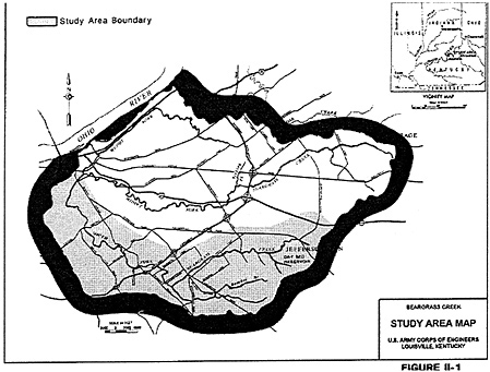
FIGURE 5.1 The Beargrass Creek basin in Louisville, Kentucky. SOURCE: USACE (1997a) (Figure II-1).

about 300 buildings and cause about $7 million in flood damages, while a 100-year flood will impact about 750 buildings and cause about $45 million in flood damages (USACE, 1997c). The expected annual flood damage under existing conditions is approximately $3 million per year.

Flood Damage Reduction Measures

Beargrass Creek has several flood damage reduction structures, the most notable of which is a very large levee at its outlet on the Ohio River ( Figure 5.2a ). This levee was built following a disastrous flood on the Ohio in January 1937, and the levee crest is an elevation of 3 feet above the 1937 flood level on the Ohio River. During the 1937 flood it was reported that “at the Public Library, the flood waters reached a height such that a Statue of Lincoln appeared to be walking on water!” (USACE, 1997b, p. III-2). Near the mouth of Beargrass Creek, a set of

gates can be closed to prevent water from the Ohio River from flowing back up into Louisville. In the event of such a flood, a massive pump station with a capacity of 7,800 cubic feet per second (cfs) is activated to discharge the flow of Beargrass Creek over the levee and into the Ohio River.

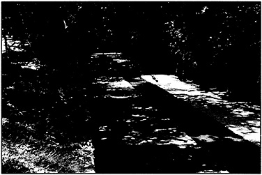
Between 1906 and 1943, a traditional channel improvement project was constructed on the lower reaches of the South Fork of Beargrass Creek. It consists of a concrete lined rectangular channel with vertical sides, with a small low-flow channel down the center ( Figure 5.2b ). The channel's flood conveyance capacity is perhaps twice that of the natural channel it replaced, but the concrete channel is a distinctive type of landscape feature that environmental concerns will no longer permit. Other structures have been added since then, including a dry bed reservoir completed in 1980, which functions as an in-stream detention basin during floods.

The proposed flood damage reduction measures for Beargrass Creek form an interesting contrast to traditional approaches. The emphasis of the proposed measures is on altering the natural channel as little as possible and detaining the floodwaters with detention basins. These basins are either located on the creek itself or more often in flood pool areas adjacent to the creek into which excessive waters can drain, be held for a few hours until the main flood has passed, and then gradually return to the creek. Figure 5.2c shows a grassed detention pond area with a concrete weir (in the center of the picture) adjacent to the creek. Figure 5.2d shows Beargrass Creek at this location (a discharge pipe from the pond is visible on the right side of the photograph). Water flows from the creek into the pond over the weir and discharges back into the creek through the pipe. The National Economic Development flood damage reduction alternative on Beargrass Creek called for a total of eight detention basins, one flood wall or levee, and one section of modified channel. Other alternatives such as flood-proofing, flood warning systems, and enlargement of bridge openings were considered but were not included in the final plan.

The evolution of flood damage reduction on Beargrass Creek represents an interesting mixture of the old and the new—massive levees and control structures on the Ohio River, traditional approaches (the concrete-lined channel) in the lower part of the basin, more modern instream and off-channel detention basins in the upstream areas, and local channel modifications and floodwalls. Maintenance and improvement of stormwater drainage facilities in Beargrass Creek are the responsibility of the Jefferson County Metropolitan Sewer District, which is the principal local partner working with the Corps to plan and develop flood damage reduction measures.

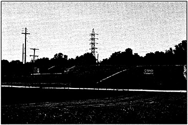
(a) Levee on the Ohio River

(b) Concrete-lined channel

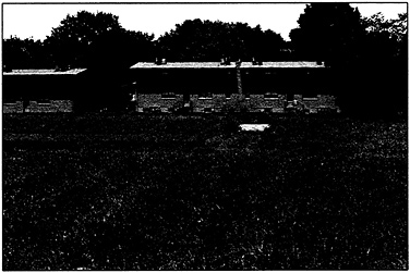
(c) Detention pond

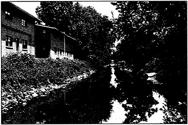
(d) Beargrass Creek at the detention pond

FIGURE 5.2 Images of Beargrass Creek at various locations: (a) the levee on the Ohio River, (b) a concrete-lined channel, (c) a detention pond, and (d) the Beargrass Creek at the detention pond.

In some locations, development has been prohibited in the floodway; but in other places, buildings are located adjacent to the creek. The Corps's feasibility report includes the following comments: “Urbanization continues to alter the character of the watershed as open land is converted to residential, commercial and industrial uses. The quest for open area residential settings in the late 1960s and early 1970s caused a tremendous increase in urbanization of the entire basin. Several developers have utilized the aesthetic beauty of the streambanks as sites for residential as well as commercial developments. This has resulted in increased runoff throughout the drainage area as development has occasionally encroached on the floodplain and, less frequently, the floodway” (USACE, 1997b, p. II-2).

Damage Reaches

To conduct the flood damage assessment, the two main creeks— South Fork of Beargrass Creek and Buechel Branch—are divided into damage reaches. Flood damage and risk assessment results are summarized for each damage reach, and the expected annual damage for the project as a whole is found by summing the expected annual damages for each reach. As shown in Figure 5.3 , the South Fork was divided into 15 damage reaches and the Buechel Branch into 5 reaches (a sixth damage reach on Buechel Branch is not shown in this figure). Approximately 12 miles of Beargrass Creek, and 2.2 miles of Buechel Branch are covered by the these damage reaches. The average length of a damage reach is thus 0.8 miles for the South Fork of the Beargrass Creek, and the average length for Buechel Branch is 0.4 miles. The shorter reaches on Buechel Branch are adjacent to similarly short, upstream reaches in Beargrass Creek where most flood damage occurs. Longer damage reaches are used downstream on Beargrass Creek where less damage occurs.

The highest expected annual flood damage is on Reach SF-9 on the upper portion of the South Fork of Beargrass Creek. Results from this damage reach are used for illustrative purposes at various points in this chapter.

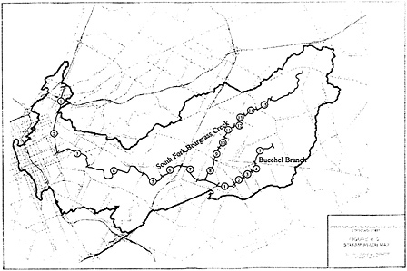
FIGURE 5.3 Damage reaches on the South Fork of Beargrass Creek and Buechel Branch. SOURCE: USACE (1997a) (Figure III-3).

Flood Hydrology

Most of the flood damage reduction measures being considered are detention basins, which diminish flood discharge by temporarily storing floodwater. It follows that the study's flood hydrology component has to be conducted using a time-varying rainfall–runoff model because this allows for the routing of storage water through detention basins. In this case, the HEC-1 rainfall–runoff model from the Corps's Hydrologic Engineering Center (HEC) was used to quantify the flood discharges. The Hydrologic Engineering Center has subsequently released a successor rainfall-runoff model to HEC-1, called HEC-HMS (Hydrologic Modeling System), which can also be used for this type of study (HEC, 1998b).

In each damage reach, and for each alternative plan considered, the risk analysis procedure for flood damage assessment requires a flood – frequency curve defining the annual maximum flood discharge at that location which is equaled or exceeded in any given year with a given probability. In this study all these flood–frequency curves were produced through rainfall–runoff modeling. In other words, a storm of a given

return period was used as input to the HEC-1 model, the water was routed through the basin, and the magnitude of the discharge at the top end of each damage reach was determined (Corps hydrologists have assumed, based on experience in the basin, that storms of given return periods produce floods of the equivalent return period). By repeating this exercise for each of the annual storm frequencies to be considered, a flood–frequency curve was produced for each damage reach. There are eight standard annual exceedance probabilities normally used to define this frequency curve: p = 0.5, 0.2, 0.1, 0.04, 0.02, 0.01, 0.004, and 0.002, corresponding to return periods of 2, 5, 10, 25, 50, 100, 250, and 500 years, respectively. In this study, because even small floods cause damage, a 1-year return period event was included in the analysis and assigned an exceedance probability of 0.999.

Considering that there are 21 damage reaches in the study area and 8 annual frequencies to be considered, each alternative plan considered requires the development of 21 flood–frequency curves involving 168 discharge estimates. During project planning, as dozens of alternative components and plans were considered, the sheer magnitude of the tasks of hydrologic simulation and data assembly becomes apparent.

The hydrologic analysis is further complicated by the fact that the design of detention basins is not simply a cut-and-dried matter. A basin designed to capture a 100-year flood requires a high–capacity outlet structure. Such a basin will have little impact on smaller floods because the outlet structure is so large that smaller events pass through almost unimpeded. If smaller floods are to be captured, a more confined outlet structure is needed, which in turn increases the required storage volume for larger floods. This situation was resolved in the Beargrass Creek study by settling on a 10-year flood as the nominal design event for sizing flood ponds and outlet works. The structures designed in this manner were then subjected to the whole range of floods required for the economic analysis.

Rainfall–Runoff Model

The HEC-1 model was validated by using historical rainfall and runoff data for four floods (March 1964, April 1970, July 1973, February 1990). Modeling results were within 5 percent to 10 percent of observed flows at two U.S. Geological Survey (USGS) streamflow gaging stations: South Fork of Beargrass Creek at Trevallian Way and Middle Fork

of Beargrass Creek at Old Cannons Lane, which have flow records beginning in 1940 and 1944, respectively, and continuing to the present. A total of 42 subbasins were used in the HEC-1 model, and runoff was computed using the U.S. Soil Conservation Service (renamed the Natural Resources Conservation Service in 1994) curve number loss rates and unit hydrographs. The Soil Conservation Service curve numbers were adjusted to allow the matching of observed and modeled flows for the historical events. A 6-hour design storm was used, which is about twice the time of concentration of the basin. The design storm duration chosen is longer than the time of concentration of the basin so that the flood hydrograph has time to rise and reach its peak outflow at the basin outlet while the storm is still continuing. If the design storm is shorter than the time of concentration, rainfall could have ceased in part of the basin before the outflow peaks at the basin outlet. The storm rainfall hydrograph was based on National Weather Service 1961 Technical Paper 40 (NWS, 1961) and on a Soil Conservation Service storm hydrograph, and a 5-minute time interval of computation was used for determining the design discharges.

There is a long flood record of 56 years of data (1940–1996) available in the study area (USGS gage on the South Fork of Beargrass Creek at Trevallian Way). A comparison was made of observed flood frequencies at this site with those simulated by HEC-1, with some adjustment of the older flood data to allow for later development. Traditional flood frequency analysis of observed flow data had little impact in the study. This may have been the case because there was only one gage available within the study area, or because the basin has changed so much over time that the flood record there does not represent homogeneous conditions. Furthermore, the alternatives mostly involve flood storage, which requires computation of the entire flood hydrograph, not just the peak discharge.

Uncertainty in Flood Discharge

Uncertainty in flood hydrology is represented by a range in the estimated flood–frequency curve at each damage reach. In the HEC-FDA program, there are two options for specifying this uncertainty: an analytical method based on the log-Pearson distribution and a more approximate graphical method. The log-Pearson distribution is a mathematical function used for flood–frequency analysis, the parameters of which are determined from the mean, standard deviation, and coefficient

of skewness of the logarithms of the annual maximum discharge data. The graphical method is a flood frequency analysis performed directly on the annual maximum discharge data without fitting them with a mathematical function. In this case the graphical method was used with an equivalent record length of 56 years of data, the length of the flood record of the USGS gage station at Trevallian Way at the time of the study. Figure 5.4 shows the flood–frequency curve for damage reach SF-9 on the South Fork of Beargrass Creek, with corresponding confidence limits based on ± 2 standard deviations about the mean curve.

The confidence limits in this graph are symmetric about the mean when the logarithm to base 10 of the discharge is taken, rather than the discharge itself. This can be expressed mathematically as:

where Q is the discharge value at the confidence limit, log Q is the expected flood discharge, σ log Q is the standard deviation (shown in the rightmost column of Table 5.1 ), and K is the number of standard deviations above or below the mean that the confidence limit lies. Because these confidence limits are defined in the log space, it follows that they are not symmetric in the real flood discharge space. As Table 5.1 shows, the expected discharge for the 100-year flood ( p = 0.01) is 4,310 cfs, the upper confidence limit is 6,176 cfs, and the lower limit is 3,008 cfs. The difference between the mean and the upper confidence limit is thus about 40 percent larger than the difference between the mean and the lower confidence limit. The confidence limits for graphical frequency analysis are computed using a method based on order statistics, as described in USACE (1997d). In this method, a given flood discharge estimate is considered a sample from a binomial distribution, whose parameters p and n are the nonexceedance probability of the flood and the equivalent record length of flood observations in the area, respectively. In this case, n = 56 years, since this is the record length of the Trevallian Way gage.

River Hydraulics

Water surface profiles for all events were determined using the HEC-2 river hydraulics program from the Corps's Hydrologic Engineering Center in Davis, California. Field-surveyed cross sections were obtained

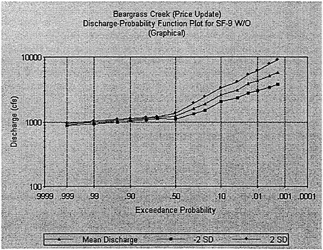
FIGURE 5.4 The flood–frequency curve and its uncertainty at damage reach SF-9 on the South Fork of Beargrass Creek.

at all bridges and at some stream sections near bridges. Maps with a scale of 1 inch = 100 feet with contour intervals of 2 feet were used to define cross sections elsewhere on the stream reaches and were used for measuring the distance between cross sections on the channel and in the left and right overbank areas. Manning's n values for roughness were based on field inspection, on reproduction of known high-water marks from the March 1964 flood on Beargrass Creek, and on reproduction of the rating curve of the USGS gage at Trevallian Way. Manning's equation relates the channel velocity to the channel's shape, slope, and roughness. Manning's n is a numerical value describing the channel roughness. Manning's n values in the concrete channel ranged from 0.015 at the channel invert to 0.027 near the top of the bank. In the natural channels, Manning 's n values ranged from 0.035 to 0.050. In the overbank areas, these values ranged from 0.045 to 0.065. Where buildings blocked the flow, the cross sections were cut off at the effective

TABLE 5.1 Uncertainties in Estimated Discharge Values at Reach SF-9

flow limits. A total of 201 cross sections were used for the South Fork of Beargrass Creek, and 61 cross sections were used for Buechel Branch. The average distance between cross sections was 330 feet on the South Fork of Beargrass Creek and 245 feet on Buechel Branch. Cross sections are spaced more closely than this near bridges and more sparsely in reaches where the cross section is relatively constant.

Figure 5.5 shows the water surface profiles along Beargrass Creek for the eight flood frequencies considered, under existing conditions without any planned control measures. The horizontal axis of this graph is the distance in miles upstream from Beargrass Creek's outlet on the Ohio River. The vertical axis is the elevation of the water surface in feet above mean sea level. The bottom profile in this graph is the channel invert or channel bottom elevation. The top profile is for p = 0.002—the 500-year flood. This particular profile shows a sharp drop near the bottom end of the channel, caused by a bridge at that location that constricts the flow. The flat water surface elevation upstream of the bridge is a backwater effect produced by the inadequate capacity of the bridge opening to convey the flow that comes to it.

For each flood profile computed, the number of structures flooded and the degree to which they are flooded must be assessed. Figure 5.6 shows the locations of the first-floor elevations of structures affected by flooding on the South Fork of Beargrass Creek in relation to several flood water surface profiles under existing conditions. Damage reach SF-9 is located between river miles (RM) 9.960 and 10.363, near the point where there is a sharp drop in the channel bed and water surface elevation on Beargrass Creek. It can be seen that the density of development varies along the channel. Flood damage reduction measures are most effective when they are located close to damage reaches with significant numbers of structures, and they are least effective when they are distant from such reaches.

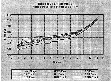
FIGURE 5.5 Water surface profiles for design floods in Beargrass Creek under existing conditions.

Each damage reach has an index location, which is an equivalent point at which all of the damages along the reach are assumed to occur. On reach SF-9, this index location is at river mile 10.124. To assess damages to structures within each reach, an equivalent elevation is found for each structure at the index location such that its depth of flooding at that location is the same as it would have been at the correct location on the flood profile, as shown in Figure 5.7 .

The technique of assigning an elevation at the index location can be far more complex than Figure 5.7 implies, because allowance is made in the HEC-FDA program for the various flood profiles to be nonparallel and also to change in gradient upstream of the index location compared to downstream. In the Beargrass Creek study, a single flood profile for the p = 0.01 event was chosen, and all other profiles were assumed parallel to this one. One damage reach on Beargrass Creek was subdivided into three subreaches to make this assumption more nearly correct. A spatial distribution of buildings over the damage reach is thus converted

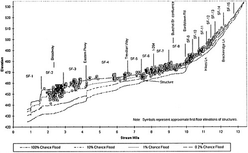
FIGURE 5.6 Locations of structures on floodwater surface profiles along the damage reaches of the South Fork of Beargrass Creek. SOURCE: USACE, 1997c.

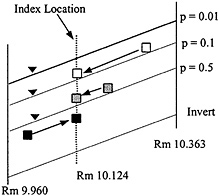
FIGURE 5.7 Assignment of structures to an index location.

into a probability distribution of buildings at the index location, where the uncertainty in flood stage is quantified.

Uncertainty in Flood Stage

The uncertainty in the water surface elevation was quantified by assuming that the standard deviation of the elevation at the index location for the 100-year discharge is 0.5 feet. The 100-year discharge at reach SF-9 is 4,310 cfs, which is the next to last set of points in Fugure 5.8 . To the right of these points, between the 100-year and 500-year flood discharges, the uncertainties are assumed to be constant. For discharges lower than the 100-year return period, the uncertainties in stage height are reduced linearly in proportion to the depth of water in the channel. The various lines shown in Figure 5.8 are drawn as the expected water surface elevation ± 1 or 2 standard deviations determined in this manner.

Economic Analysis

The Corps's analysis of a flood damage reduction project's economic costs and benefits is guided by the Principles and Guidelines ( Box 1.1 provides details on the P&G's application to flood damage reduction

FIGURE 5.8 Uncertainty in the flood stage for existing conditions at reach SF-9 of the South Fork of Beargrass Creek.

studies). According to the P&G , the economic analysis of damages avoided to floodplain structures because of a flood damage reduction project is restricted to existing structures (i.e., federal policy does not allow damages avoided to prospective future structures to be counted as benefits). The P&G do, however, call for the benefits of increased net income generated by floodplain activities after a project has been constructed (so-called “intensification benefits”) to be included in the economic analysis.

Economic analysis of flood damages considers various sorts of flood damage, principal among them being the damage to flooded structures. Information about the structures is quantified using a “structure inventory,” an exhaustive tabulation of every building and other kind of structure subjected to flooding in the study region. A separate computer program called Structure Inventory for Damage Analysis (SID) was used

to evaluate the number of structures flooded as a function of water surface elevation. Structures are divided into four categories: single-family residential, multifamily residential, commercial, and public. A structure is considered to be flooded if the computed flood elevation is above its first-floor elevation. The amount of damage D is a function of the depth of flooding h and the type of structure, and is expressed by a factor, r ( h ), which is equal to a percentage of the value of the structure ( V ) and of its contents (C). This analysis can be expressed as

D = r 1 ( h ) V + r 2 ( h ) C . (5.2)

For residential structures, these damage factors were quantified in 1995 by the Federal Emergency Management Agency (FEMA) using data from flood damage claims. For example, for a one-story house without a basement flooded to a depth of 3 feet, the FEMA estimate is that the damage factors are r 1 = 27% of the value of the structure and r 2 = 35% of the value of the contents. For the same house flooded to a depth of 6 feet, the corresponding damage factors are r 1 = 40% for the structure, and r 2 = 45% for the contents, respectively. The Marshall and Swift Residential Cost Handbook (Marshall and Swift, 1999) was used to estimate the value of single- and multi-family structures (it bears mentioning that the use of standard references such as the Marshall and Swift handbook may potentially represent another source of “knowledge uncertainty ”). The values of their contents were assumed to be 40 percent to 44 percent of the value of the structure. For commercial and public buildings, the values of the structures and their contents were established through personal interviews by Corps personnel. About 85 percent of the structures subject to flood damage are residential buildings.

Types of flood damages beyond those to structures were also considered. For instance, there are several automobile sales lots in the floodplain, and prospective damages to cars parked there during a flood were estimated. Nonphysical damage costs include the costs of emergency services and traffic diversion during flooding. Damage to roads and utilities were also considered.

Uncertainty in Flood Damage

The economic analysis has three sources of uncertainty:

the elevation of the first floor of the building,

the degree of damage given the depth of flooding within the building, and

the economic value of the structure and its contents.

For most structures in Beargrass Creek, the first-floor elevation was estimated from the ground elevation on maps with a scale of 1 inch = 100 feet and with contour intervals of 2 feet. For a sample of 195 structures (16% of the total number), the first-floor elevations were surveyed. It was found that the average difference between estimated and surveyed first-floor elevations of these structures was 0.62 feet.

Corps Engineering Manual (EM) 1110-2-1619 (USACE, 1996b) was used to estimate values for the uncertainties in economic analysis. A standard deviation of 0.2 feet was used to define the uncertainty in first-floor elevations. The uncertainty in the degree of damage given a depth of inundation was estimated by varying the percent damage factor described previously. For residential structures the value of the structure was assigned a standard deviation of 10 percent of the building value, and the ratio of the value of the contents to the structure was allowed to vary with a standard deviation of 20 percent to 25 percent.

For commercial property a separate damage estimate, based on interviews with the owners, was made for each significant property and was expressed as a triangular distribution with a minimum, expected, and maximum damage value for the property. Because every individual structure potentially affected by flooding is inventoried in the damage estimate data, the amount of work required to collect all these damage data was extensive.

The end result of these estimates at each damage reach and damage category is a damage–stage curve (such as Figure 5.9 ) that accumulates the damage to all multifamily structures in this damage reach for various water surface elevations at the index location, denoted by stage on the horizontal axis. This curve is prepared by first dividing the range of the stage (476–486 feet) into increments —increments of 0.5 feet in this case. For each structure, a cycle of 100 Monte Carlo simulations is carried out in which the first-floor elevation and the values of the structure and contents are randomly varied. From these simulations estimates are formed for each 0.5-foot stage height increment of what the expected damage and standard deviation of the damage to that structure would be if the flood stage were to rise to that elevation. For each stage increment, these means and standard deviations are accumulated over all structures in the

reach to form the estimate of the mean and standard deviation of the reach damage ( Figure 5.9 ).

A similar function is prepared for each of the damage categories. At any flood stage, the sum of the damages across all categories is the total flood damage for that reach.

Project Planning

The discussion of the Beargrass Creek study reviewed the technical means by which a particular flood damage reduction plan is evaluated. A plan consists of a set of flood damage reduction measures, such as detention ponds, levees or floodwalls, and channel modifications, implemented at particular locations on the creek. The base plan against which all others are considered is the “without plan,” which means a plan that considers existing conditions in the floodplain and the development expected to occur even in the absence of a flood damage reduction plan. Such development must meet floodplain management policies and have structures elevated out of the 100-year floodplain. A base year of 1996 was chosen for the Beargrass Creek study.

In carrying out project planning, the spatial location of the principal damage reaches is important because flood damage reduction measures located just upstream of or within such reaches have greater economic impact than do flood damage reduction measures located in areas of low flood damage. Project planning also involves a great deal of interaction with local and state agencies, in this case principally the Jefferson County Metropolitan Sewer District.

The Beargrass Creek project planning team consisted primarily of three individuals in the Corps's Louisville district office: a project planner from the planning division, a hydraulic engineer from the hydrology and hydraulics design section, and an economic analyst from the economics branch. The HEC-FDA computer program with risk analysis was carried out by the economic analyst using flood–frequency curves and water surface profiles supplied by the hydrology and hydraulics section and using project alternatives defined by the project planner. The hydrology and hydraulics section was also responsible for the preliminary sizing of potential project structures being considered as plan components. The bulk of the work of implementing the risk analysis aspects of flood damage assessment thus fell within the domain of the Corps economic analyst.

The HEC-FDA program is applied during the feasibility phase of

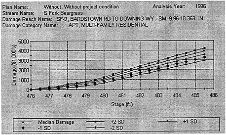
FIGURE 5.9 The damage–stage curve with uncertainty for multifamily residential property in Reach SF-9 of the South Fork of Beargrass Creek.

flood damage reduction planning. This had been preceded by a reconnaissance phase, a preliminary assessment of whether reasonable flood damage reduction planning can be done in the area. As explained in Chapter 2 , the reconnaissance phase is fully funded by the federal government, but the feasibility phase must have half the costs met by a local sponsor. Assuming the feasibility phase yields an acceptable plan and additional funds are authorized, the project proceeds to a detailed design and construction phase, which also requires local cost sharing. The Beargrass Creek project is now (as of May 2000) in the detailed design phase.

Evaluation of Project Alternatives

Expected annual flood damages in Beargrass Creek under existing conditions are estimated to be $3 million. Project benefits are calculated as the difference between this figure and the lower expected annual damages that result with project components in place. Project costs are annualized values of construction costs discounted over a 50-year period using an interest rate of 7.625 percent. Project net benefits are the differ-

ence between project benefits and costs. For components to be included in the project, they must have positive net benefits.

The first step in evaluating project alternatives is to consider each component flood damage reduction measure by itself to see if it yields positive net benefits. A total of 22 components were examined individually, 11 on the South Fork of Beargrass Creek and 11 on Buechel Branch. All 11 of the South Fork components were economically justified on a stand-alone basis. Only 3 of the 11 components on Buechel Branch were justified individually: the other 8 components were thus deleted from further consideration.

The next step is to formulate the National Economic Development (NED) plan. In theory, this is supposed to proceed by selecting first the component with the largest net benefits, adding the component with the next largest net benefits, evaluating them together, and continuing to add more components until the combined set of components has the largest overall net benefits. It turned out that this idealized approach could not be used at the South Fork of Beargrass Creek because of economic and hydraulic interactions among the components. The study team commented: “Therefore, the formulation process was different and more complicated than originally anticipated. The study team could not follow the incremental analysis procedure to build up the NED plan because the process became a loop of H&H computer runs. Our component with the greatest net benefits is located near the midpoint of the stream; thus, each time we would add a component upstream it would affect all components downstream and vice versa. We could never truly optimize or identify the plan which produces the greatest net benefits” (USACE, 1997c, p. IV-62).

The problems were further complicated by the fact that there are three separate sections of the study region: the South Fork of Beargrass Creek and Buechel Branch upstream of their junction and the South Fork downstream of this junction ( Figure 5.3 ). In the downstream region, flood damage reduction measures on the upper South Fork and Buechel Branch compete for project benefits by reducing flood damages. The result of these complications is that the plan was built up incrementally by separately considering the three sections of the region. First, the most upstream control structure in each section was selected, then structures downstream were added. At the end—when the components from the three sections had been aggregated into a single overall plan—it was determined whether the plan could be improved by omitting individual marginal components. The end result of this iterative process was a recommended plan with 10 components: 8 detention basins, 1 floodwall,

and 1 channel improvement.

Each plan has to be evaluated using the Monte Carlo simulation process. The number of simulations varies by reach, with 10,000 required for Reach SF-9 and with a range of 10,000–100,000 required for the other reaches. On a 300 MHz Pentium computer, evaluation of a single plan takes about 25 minutes of computation time.

Risk of Flooding

The HEC-FDA program also produces a set of statistics that quantify the risk of being flooded in any reach for a given plan, as shown in Table 5.2 . For reach SF-9, the target elevation is 477.2 feet, which is the elevation of the overbank area in this reach. The probability estimates shown are annual exceedance probability and conditional nonexceedance probability. The annual exceedance probability refers to the risk that flooding will occur considering all possible floods in any year. The conditional nonexceedance probability describes the likelihood that flooding will not occur during a flood of defined severity, such as the 100-year (1 percent chance) flood.

There is a subtle but important distinction between these two types of risk measures. The annual exceedance probability accumulates all the uncertainties into a single estimate both from the natural variability of the unknown severity of floods and from the knowledge uncertainty in estimating methods and computational parameters. The conditional non-exceedance probability estimate divides these two uncertainties, because it is conditional on the severity of the natural event and thus represents only the knowledge uncertainty component. In this sense, the conditional nonexceedance probability corresponds most closely to the traditional idea of adding 1 foot or 3 feet on the 100-year base flood elevation, while the annual exceedance probability corresponds more closely to the goal of ensuring that the chance of being flooded is less than a given value, such as 1 percent, considering all sources of uncertainty.

The “target stage annual exceedance probability” values in Table 5.2 are the median and the expected value or mean of the chance that flooding will occur in any given year for the various reaches. Thus, for reach SF-9, there is approximately a 36 percent chance that flooding will occur beyond the target stage in any given year, while in reach SF-14 upstream, that chance is only about 9 percent. The “long term risk” values in the

TABLE 5.2 Risk of Flooding in Damage Reaches Calculated Uncertainty for 1996 at Beargrass Creek

figure refer to the chance (Rn) that there will be flooding above the target stage at least once in n years, determined by the formula

R n = 1− (1− p e ) n , (5.3)

where p e is the expected annual exceedance probability. For example, for reach SF-9, where p e = 0.3640, for n = 10 years, R 10 = 1− (1 − 0.3640) 10 = 0.9892, as shown in Table 5.2 .

The conditional nonexceedance probability values shown on the right-hand side of Table 5.2 are conditional risk values that correspond to the reliability that particular floods can be conveyed without causing damage in this reach. Thus, in reach SF-9, a 10 percent chance event (10-year flood) has about a 0.27 percent chance of being conveyed without exceeding the target stage, while for a 1 percent chance event (100-year flood), there is essentially no chance that it will pass without exceeding the target stage. By contrast, in Reach SF-14 at the upstream end of the study area, the conditional nonexceedance probability of the reach passing the 10-year flood is about 52 percent; that of the reach passing the 100-year flood is about 100 percent. As the flood severity increases, the chance of a reach being passed without flooding diminishes.

Effect on Project Economics of Including Risk and Uncertainty

The HEC-FDA program that includes risk and uncertainty factors in project analysis became available to the Beargrass creek project team late in the study period. Before then, the team used an earlier economic analysis program (Expected Annual Damage, or EAD) which computed expected annual damages without these uncertainties. O' Leary (1997) presented the data shown in Table 5.3 to compare the two approaches. It is evident that including risk and uncertainty increases the expected annual damage both with and without flood damage reduction plans. The net effect of their inclusion on the Beargrass Creek project is to increase the annual flood damage reduction benefits from $2.078 million to $2.314 million. The study team made a comparison between the components included in the National Economic Development plan in the two computer programs and found that there was no change. Hence, although the inclusion of risk and uncertainty increased project benefits, it did not result in changing the flood damage reduction components included in the National Economic Development plan.

O'Leary (1997) also presented statistics of the project benefits derived from the HEC-FDA program for the National Economic Development plan. The expected annual benefits of the National Economic Development plan—$2.314 million—are the same in Table 5.3 and Table 5.4 . The net benefits in the fourth column of Table 5.4 are found by subtracting the annual project costs from the expected annual benefits; the benefit-to-cost ratio is the ratio of the expected benefits to costs.

The 25 th percentile, median (50 th percentile), and 75 th percentile of the expected annual benefits are also shown. The project net benefits are positive at all levels of assessment, and all benefit-to-cost ratios are greater than 1.00. It is interesting to see that the median expected annual benefits ($2.071 million) are nearly the same as the expected value of these benefits without considering uncertainty ($2.078 million). Moreover, the expected value ($2.314 million) is greater than the median, and the difference between the 75 th percentile and the median is greater than the difference between the median and the 25 th percentile. All these characteristics point to the fact that the distributions of flood damages and of expected annual benefits are positively skewed when uncertainties in project hydrology, hydraulics, and economics are considered. This is why the project benefits increase when these uncertainties are considered. The project benefits for the 25 th percentile, 50 th percentile, and 75 th percentile in Table 5.4 should be read with caution because they are compiled for the project by adding together the corresponding values for all the damage reaches. The percentile value of a sum of random variables is not necessarily equal to the sum of the percentile values of each variable.

TABLE 5.3 Expected Annual Damages (EAD) With and Without Uncertainty in Damage Computations (millions of dollars per year)

TABLE 5.4 Statistics of project benefits under the NED plan using the HEC-FDA Program

RED RIVER OF THE NORTH AT EAST GRAND FORKS, MINNESOTA, AND GRAND FORKS, NORTH DAKOTA

A devastating flood occurred at East Grand Forks, Minnesota, and Grand Forks, North Dakota, in April 1997. After the flood, flood damage reduction studies previously done for the two cities were combined into a joint study, and risk analysis was performed to evaluate the reliability of the proposed alternatives and to evaluate their economic impacts. A risk analysis study performed before the flood was presented in a paper at the Corps's 1997 Pacific Grove, California, workshop (Lesher and Foley, 1997). This paper and subsequent analysis (USACE, 1998a, b, c), as well as a visit to the Corps's St. Paul district office by a member of this committee, form the basis of this discussion of the East Grand Forks–Grand Forks study.

East Grand Forks, Minnesota, and Grand Forks, North Dakota, are located on opposite banks of the Red River of the North and are approximately 300 miles above the river's mouth at Lake Winnipeg, Manitoba, Canada ( Figure 5.10 ). The East Grand Forks–Grand Forks metropolitan area has a population of approximately 60,000 and is located about 100 miles south of the U.S.–Canadian border. The total drainage area of the East Grand Forks–Grand Forks basin is 30,100 square miles. Included in this drainage area is the Red Lake River subbasin that effectively drains about 3,700 square miles in Minnesota and joins the mainstream of the Red River at East Grand Forks. The study area of East Grand Forks–Grand Forks lies in the middle of the Red

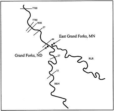
FIGURE 5.10 Schematic of the Red River of the North (RRN) and Red Lake River (RLR) at the East Grand Forks, Minnesota and Grand Forks, North Dakota study area. Numbers indicate USGS stream gages.

River Valley. The valley is exceptionally flat with a gradient that slopes 3–10 feet per mile toward the river with the north–south axis having a gradient of about three-quarters of a foot per mile. The valley extends approximately 23 miles west and 35 miles east of East Grand Forks– Grand Forks and is a former glacial lake bed.

Both cities have a long history of significant flooding from the Red River of the North and the Red Lake River. The most damaging flood of record occurred in April 1997 (see Table 5.5 ), when the temporary levee systems and flood-fighting efforts of both communities could not hold back the floodwaters of the Red River. The resulting damages were disastrous and affected both cities dramatically. Total damages to existing structures and contents during the 1997 flood were estimated to exceed $800 million. An additional $240 million was spent for emergency-related costs.

TABLE 5.5 Maximum Recorded Instantaneous Peak Flows; Red River of the North at Grant Forks, North Dakota

Risk Analysis

A risk analysis for the proposed flood damage reduction project for the Red River of the North at East Grand Forks, Minnesota, and Grand Forks, North Dakota, used a Latin Hypercube analysis to sample interactions among uncertain relationships associated with flood discharge and elevation estimation. Latin Hypercube is a stratified sampling technique used in simulation modeling. Stratified sampling techniques, as opposed to Monte Carlo-type techniques, tend to force convergence of a sampled distribution in fewer samples. Because the Hydrologic Engineering Center Flood Damage Analysis program (HEC-FDA) was new at the time, and in the interest of saving time, the analysis was performed using a spreadsheet template. The flood damage reduction alternatives analyzed included levees of various heights and a diversion channel in conjunction with levees. The project reliability option in the HEC risk spreadsheet was used to determine the reliability of the alternative levee heights and of the diversion channel in conjunction with levees. The following sections discuss the sensitivity in quantifying the uncertainties and the representation of risk for the alternatives.

Discharge–Frequency Relationships

The log-Pearson Type III distribution, recommended in the Water Resource Council's Bulletin 17B (IACWD, 1981) and incorporated

within the Corps's HEC Flood Frequency Analysis (HEC-FFA) computer program, was used for frequency analysis of maximum annual streamflows, and the noncentral t distribution was used for the development of confidence limits. Discharge–frequency relationships were needed for both the levees and the diversion channel in combination with levees. An analysis (coincidental frequency) was performed to develop the discharge– frequency curves for the Red River of the North downstream and upstream of the Red Lake River for the levees only condition. A graphical method was used to develop the discharge–frequency curves for the diversion channel in combination with levees. Details of these procedures can be found in a Corps instruction manual from the St. Paul district (USACE, 1998a). A brief discussion of these procedures is provided below.

The Grand Forks USGS stream gage (XS 44) is currently located 0.4 miles downstream from the Red Lake River in Grand Forks, North Dakota ( Figure 5.10 ). The discharge–frequency curve for this station along with the 95 percent and 5 percent confidence limits (90% confidence band) are plotted in Figure 5.11 . An illustration of the noncentral t probability density function for the 1 percent event is also shown in that figure. Selected quantities of that discharge–frequency relationship are shown in column 2 of Table 5.6 . The coincidental discharge–frequency relationship for the Red River just upstream of the mouth of the Red Lake River (column 3 of Table 5.6 ) was computed with the HEC-FFA computer program. The basic flow values were obtained by routing the 96 years of available data on Red Lake River flows from Crookston (55 miles upstream of the mouth) downstream to Grand Forks. The resulting flows were subtracted from the Red River at Grand Forks flows to obtain coincident discharges on the Red River upstream of Red Lake River. The two-station comparison method of Bulletin 17B was used to adjust the logarithmic mean and standard deviation of this short record (96 years) based on regression analysis with the long-term record at the Grand Forks station (172 years). Correlation of coincident flows for the short record with concurrent peak flows for the long record produced a correlation coefficient of 0.975.

Adjustment of the statistics yielded an equivalent record length of 165 years. The adopted coincidental discharge–frequency curve for the Red River upstream of the Red Lake River is shown in column 3 of Table 5.6 for selected annual exceedance probabilities. The coincidental discharge –frequency curve for the Red Lake River at the mouth was determined by computing the difference in Red River flows both upstream and downstream of Red Lake River (see column 4 in Table 5.6 ). Statistics for the adopted relationship were approximated by synthetic methods presented in Bulletin 17B (for more details, see USACE (1998a)).

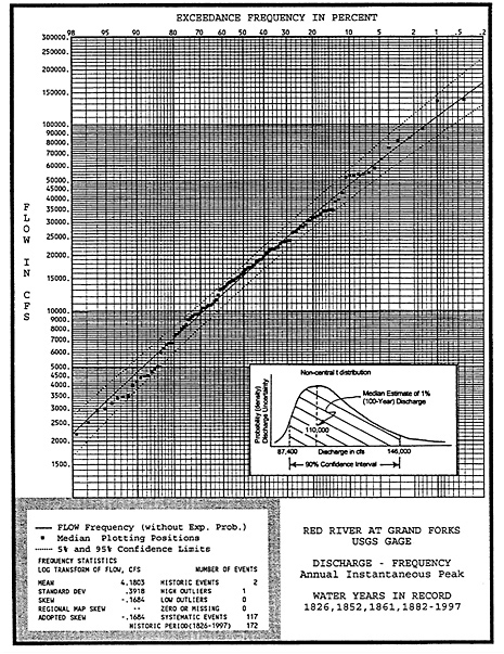
FIGURE 5.11 Flood (discharge) frequency curve for the Red River at Grand Forks.

TABLE 5.6 Instantaneous Annual Peak Discharges (cfs) and their Annual Exceedance Probabilities (%) — Existing Conditions

and downstream of Red Lake River (see column 4 in Table 5.6). Statistics for the adopted relationship were approximated by synthetic methods presented in Bulletin 17B (for more details, see USACE (1998a)).

The Plan Comparison Letter Report developed in February 1998 for flood damage reduction studies for East Grand Forks, Minnesota, and Grand Forks, North Dakota, evaluated an alternative flood damage reduction plan that included a split-flow diversion channel along with permanent levees. The discharge–frequency relationships for the modified conditions, shown in Table 5.7 , were developed as follows. The modified-condition discharge–frequency curve for the Red River upstream of Red Lake River was graphically developed based upon the operation of the diversion channel inlet. Red River flows are not diverted until floods start to exceed those having return periods of 5 years (20% annual exceedance probability). The channel is designed to continue to divert Red River flows at a rate that allows the design flood (0.47%) discharge of 102,000 cfs (upstream of the diversion) to be split such that 50,500 cfs is diverted and 51,500 cfs is passed through the cities. This operation is reflected in the modified discharge–frequency relationship shown in Table 5.7 for the Red River upstream of Red Lake River (columns 2 and

TABLE 5.7 Instantaneous Annual Peak Discharges (cfs) and their Annual Exceedance Probabilities (%)—Condition with Diversion Channels

3).Synthetic statistics (mean, standard deviation, and skewness) in accordance with methodology presented in Bulletin 17B were computed for the discharge-frequency relationships of the below-diversion flows.

The modified-condition discharge–frequency curve for the Red River downstream of Red Lake River was graphically computed based upon the operation of the diversion channel. The modified-condition Red River discharges upstream of Red River were added to the coincident flows on Red Lake River (column 4). The resulting discharges were plotted for graphical development of the modified-condition discharge– frequency relationship for the Red River downstream of Red Lake River and are summarized in Table 5.7 (column 5). Synthetic statistics for this discharge–frequency relationship were computed for use in the risk analysis.

Elevation–Discharge Relationships

The water surface elevations computed using the HEC-2 computer program are shown in Table 5.8 for three cross sections (7790, 7800, and 7922) corresponding to the previous USGS gage locations and for cross

section 44, which corresponds to the current USGS gage location (see Figure 5.10 for the cross section locations). These computed water surface elevations (CWSE) were based on the expected discharge quantities from the coincidental frequency analysis performed in June 1994 for the Grand Forks Feasibility Study. These data were used to transfer observed elevations from previous USGS gage sites to the current site (cross section 44) at river mile 297.65, and they were used in determining the elevation –discharge uncertainty. The water surface profile analysis was performed using cross-sectional data obtained from field surveys. Data were also obtained from field surveys and from USGS topographic maps. The HEC-2 model was calibrated to the USGS stream gage data and to high-water marks for the 1969, 1975, 1978, 1979 and 1989 flood events throughout the study area. Note that these water surface elevations assume the existing East Grand Forks and Grand Forks emergency levees are effective. The levees were assumed effective because through extraordinary efforts, they have generally been effective for past floods with the exception of the 1997 flood.

Ratings at stream gage locations provide an opportunity to directly analyze elevation–discharge uncertainty. The measured data are used to derive the “best fit” elevation-discharge rating at the stream gage location, which generally represents the most reliable information available. In this study, the adopted rating curve for computing elevation uncertainty is based on the computed water surface elevations from the calibrated HEC-2 model shown in Table 5.8 .

This adopted rating curve for cross section 44 at the current USGS gage is shown in Figure 5.12 . Measurements at the gage location were used directly to assess the uncertainty of the elevation–discharge relationship. The normal distribution was used to describe the distribution of error from the “best-fit” elevation–discharge rating curve. The observed gage data (for the four cross sections presented in Table 5.8 ) were transferred to the current gage site at river mile 297.65 based on the gage location adjustments presented in Table 5.9 , which were computed from the water surface elevations in Table 5.8 . These adjustments were plotted against the corresponding discharge below the Red Lake River, and curves were developed to obtain adjustments for other discharges.

The deviations of the observed elevations from the fitted curve were used to estimate the uncertainty of the elevation–discharge rating curve shown in Figure 5.11 . The deviations reflect the uncertainty in data values as a result of changes in flow regime, bed form, roughness/resistance to flow, and other factors inherent to flow in natural streams. Errors also

TABLE 5.8 Computed Water Surface Elevations of the Red River of the North at Grand Forks, North Dakota (units in feet above sea level)

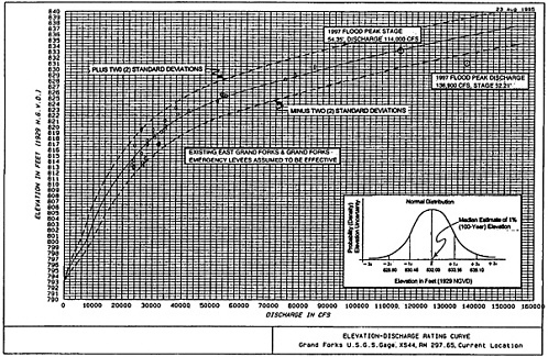
FIGURE 5.12 Rating curve (water elevation vs. discharge)for the Red River at Grand Forks.

TABLE 5.9 Adjustments Used in Transferring Observed Elevations from Previous USGS Gage Sites to Current Gage Site at RM 297.65 (XS 44)

result from field measurements or malfunctioning equipment. A minimum of 8–10 measurements is normally required for meaningful results. The measure used to define the elevation–discharge relationship uncertainty is the standard deviation:

Where X = observed elevation adjusted to current gage location (if 5.12 necessary), M = computed elevation from adopted rating curve, and N = number of measured discharge values (events).

The elevation uncertainty was computed for two different discharge ranges for this analysis. Based on the observed elevations plotted on the adopted rating curve, it appeared that there was greater uncertainty for discharges less than about 10% of annual exceedance probability event due to ice effects on flow. Therefore, the standard deviation was computed for discharges greater than between 22,000 cfs, which corresponds approximately to the zero damage elevation based on the adopted rating curve, and 44,000 cfs, which is slightly greater than the 10 percent annual exceedance probability. The standard deviation was also computed for discharges greater than 50,000 cfs. During the period of record, there were 25 events with a discharge between 22,000 and 44,000 cfs and 10 events with a discharge greater than 50,000 cfs. The standard deviation was 1.66 feet for discharges between 22,000 and 44,000 cfs and was 1.55

feet for discharges greater than 50,000 cfs. In the risk and uncertainty simulations, the standard deviation was linearly interpolated between 1.66 and 1.55 feet for discharges between 44,000 and 50,000 cfs. (See USACE (1998b) for more details.)

In an earlier risk analysis that was performed for the Grand Forks Feasibility Study, a much lower standard deviation of 0.50 feet was used for discharges greater than 50,000 cfs. However, adding the 1997 flood to the analysis resulted in a standard deviation of 1.55 feet, which is similar to that computed for discharges less than 44,000 cfs. It should be noted that the discharge and elevation used in this analysis for the 1997 flood was the peak discharge of 136,900 cfs occurring on April 18, 1997 (see Table 5.4 ), and an elevation of 831.21 feet (Stage 52.21). The peak elevation of 833.35 feet (Stage 54.35) occurred on April 22, 1997 at a discharge of 114,000 cfs. The elevation of 831.21 feet was almost 5 feet below the rating curve at a discharge of 136,900 cfs; however, the peak elevation of 833.35 feet at a discharge of 114,000 cfs was essentially on the adopted rating curve. Both of these points are plotted on the rating curve in Figure 5.12 . Lines representing ± 2 standard deviations for the normal distribution, which encompasses approximately 95 percent of all possible outcomes, are also shown on the rating curve. An illustration of the normal distribution at the 1 percent (100-year) event for the project levee condition is also shown in Figure 5.12 .

Risk and Uncertainty Analysis Results

Four index locations were selected to evaluate project performance and project sizing. These locations are cross sections 57, 44 (current USGS gage), 27, and 15 ( Figure 5.10 ). The four locations were selected based on economic requirements for project sizing (see USACE, 1998c). The elevation–discharge rating curves (based on HEC-2 analysis) for existing and project conditions at these locations can be found in the USACE (1998b). Each of these rating curves shows three conditions, where applicable: (1) existing conditions, (2) removal of the pedestrian bridge at cross sections 7920-7922 and with project levees (“levee only”); and (3) with removal of the pedestrian bridge, with project levees, and with the diversion channel (“diversion channel”). Existing conditions means that the existing emergency levees are assumed to be effective up to and including the 5 percent (20-year) event and are ineffective for larger floods. The 5 percent (20-year) event was selected based

on comparison of water surface profiles with effective and probable failure point (PFP) levee elevations provided by the Geotechnical Design Section analysis (see USACE, 1998b, paragraph A.2.11 and Appendix B of this report). The pedestrian bridge was removed based on input from the cities of East Grand Forks and Grand Forks. The rating curves for the diversion channel alternative were based on limited information. The Red River to the North would start to divert into the diversion channel at the 20 percent (5-year) flood; therefore, up to this point the rating curve for existing conditions with levees was used.

An additional location was also selected to evaluate the performance of the levee only and diversion channel with 1 percent (100-year) levee alternatives. This location is at cross section 7700 at the downstream end of the project levees (see Figure 5.10 ). Cross section 7700 was selected based on hydraulic analysis as the least critical location—the location where the levees in combination with the diversion channel would first overtop from downstream backwater (see USACE, 1998b).

Project Reliability

The project reliability results are summarized in Table 5.10 , Table 5.11 through Table 5.12 . Table 5.9 contains the results for the levees-only alternatives. Table 5.11 contains the results for the diversion channel in combination with 1 percent (100-year) levees. Note that in Table 5.10 , three different alternative top-of-levee heights are evaluated, whereas in Table 5.11 , it is always the same alternative—diversion channel with 1 percent levees— but for the three different events. The top-of-levee elevations were computed based on a water surface elevation profile to ensure initial overtopping would occur at the least-critical location (here, cross section 7700). The downstream top-of-levee elevations were selected with the intent of having 90 percent probability of containing the specified flood and were based on previous risk analysis for the Grand Forks Feasibility Study preliminarily updated to include the 1997 flood. The 2 percent (50-year), 1 percent (100-year), and 0.47 percent (210-year/1997 flood) top-of-levee profiles are 3.2, 3.4, and 2.7 feet above their respective water surface profiles at the downstream end ( Table 5.10 ).

As seen in Table 5.10 , the intent of having 90 percent probability of containing the specified flood is generally realized. The 2 percent levees have a 92 percent probability of containing the 2 percent flood. The 1 percent levees have a 90 percent probability of containing the 1 percent

flood. The 0.47 percent levees have an 87 percent probability of containing the 0.47 percent flood.

TABLE 5.10 Reliability at Top of Levee for Three Top-of-Levee Heights

TABLE 5.11 Project Reliability at Top of Levee for Diversion Channel with 1 Percent (100-Year) Levees for Three Different Events

Reliability results for the diversion channel with 1 percent levees are summarized in Table 5.11 . Note again that the levees constructed in combination with the diversion are the same as for the 1 percent flood without the diversion channel and are the same for all three floods analyzed. As seen in the table, there is a 99 percent or greater probability of containing the flood for all three floods considered when the project includes the diversion channel.

As previously noted, the most critical location for project performance is at cross section 7700 at the downstream end of the project. Table 5.12

summarizes the results for all the alternatives considered and for numerous floods. The probability of the diversion channel in combination with 1 percent levees for the 0.2 percent event is listed in the table as greater than 95%. A more specific reliability was not cited for the 0.2 percent event for two reasons: (1) the discharge–frequency curve based on the approximate statistics starts to diverge from the graphical curve for extreme events and, (2) there was limited information available to develop the Red River to the North rating curves for the diversion alternative. These reasons are also why more extreme events were not analyzed.

TABLE 5.12 Conditional Exceedance Probability of Alternative for Various Events (based on analysis at downstream end of project—XS 7700)

Table 5.13 presents the simulated conditional exceedance probabilities from the economic project sizing analysis. The without-project condition is also included in this table for comparison purposes. The without-project condition is based on a zero damage elevation of 824.5 feet, assumes credit is given to the existing levees, and assumes all properties that were substantially damaged (50% or more damage) in the 1997 flood have been removed.

Based on the above analysis of alternative plans and further economic and environmental considerations, the recommended National

TABLE 5.13 Residual Risk Comparison

Economic Development (NED) plan consists of a permanent levee and floodwall system designed to reliably contain the 210-year flood event. This equates to an 87.7 percent reliability of containing the 210-year flood event ( Table 5.12 ) and would reliably protect against a flood of the magnitude of the 1997 flood.

The recommended plan would remove protected areas from the regulatory floodplain, increase recreational opportunities, and enhance the biological diversity in the open space created. The recommended plan anticipates the need to acquire over 250 single-family residential structures, 95 apartment or condominium units, and 16 businesses along the current levee/floodwall alignment.

The total cost of the recommended multipurpose project is $350 million including recreation features and cultural resources mitigation costs. The federal share of the project would be $176 million and the nonfederal share would be $174 million. The benefit-to-cost ratio has been calculated as 1.07 for the basic flood reduction features of the project and as 1.90 for the separable recreation features (USACE, 1998b). The recommended project has an overall benefit-to-cost ratio of 1.10.

The cities of East Grand Forks, Minnesota, and Grand Forks, North Dakota, will serve as the project's nonfederal sponsors. Through legislation, the State of Minnesota has committed to provide financial support in the form of bonds and returned sales taxes to the city of East Grand Forks. In verbal and written comments from its governor, the State of North Dakota has committed to provide financial assistance to the city of Grand Forks.

Reducing flood damage is a complex task that requires multidisciplinary understanding of the earth sciences and civil engineering. In addressing this task the U.S. Army Corps of Engineers employs its expertise in hydrology, hydraulics, and geotechnical and structural engineering. Dams, levees, and other river-training works must be sized to local conditions; geotechnical theories and applications help ensure that structures will safely withstand potential hydraulic and seismic forces; and economic considerations must be balanced to ensure that reductions in flood damages are proportionate with project costs and associated impacts on social, economic, and environmental values.

A new National Research Council report, Risk Analysis and Uncertainty in Flood Damage Reduction Studies , reviews the Corps of Engineers' risk-based techniques in its flood damage reduction studies and makes recommendations for improving these techniques. Areas in which the Corps has made good progress are noted, and several steps that could improve the Corps' risk-based techniques in engineering and economics applications for flood damage reduction are identified. The report also includes recommendations for improving the federal levee certification program, for broadening the scope of flood damage reduction planning, and for improving communication of risk-based concepts.

READ FREE ONLINE

Welcome to OpenBook!

You're looking at OpenBook, NAP.edu's online reading room since 1999. Based on feedback from you, our users, we've made some improvements that make it easier than ever to read thousands of publications on our website.

Do you want to take a quick tour of the OpenBook's features?

Show this book's table of contents , where you can jump to any chapter by name.

...or use these buttons to go back to the previous chapter or skip to the next one.

Jump up to the previous page or down to the next one. Also, you can type in a page number and press Enter to go directly to that page in the book.

Switch between the Original Pages , where you can read the report as it appeared in print, and Text Pages for the web version, where you can highlight and search the text.

To search the entire text of this book, type in your search term here and press Enter .

Share a link to this book page on your preferred social network or via email.

View our suggested citation for this chapter.

Ready to take your reading offline? Click here to buy this book in print or download it as a free PDF, if available.

Get Email Updates

Do you enjoy reading reports from the Academies online for free ? Sign up for email notifications and we'll let you know about new publications in your areas of interest when they're released.

Advertisement

Understanding urban flood vulnerability and resilience: a case study of Kuantan, Pahang, Malaysia

• Original Paper
• Open access
• Published: 14 March 2020
• Volume 101 , pages 551–571, ( 2020 )

Cite this article

You have full access to this open access article

• M. Y. Safiah Yusmah   ORCID: orcid.org/0000-0002-4317-6124 1 ,
• L. J. Bracken   ORCID: orcid.org/0000-0002-1268-5516 2 ,
• Z. Sahdan 3 ,
• H. Norhaslina 1 ,
• M. D. Melasutra 4 ,
• A. Ghaffarianhoseini 1 ,
• S. Sumiliana 5 &
• A. S. Shereen Farisha 1  

14k Accesses

26 Citations

1 Altmetric

Explore all metrics

Malaysia is frequently affected by the annual flooding event caused by the seasonal monsoon which accounts for significant losses. Flood risk, exposure and damage potential are increasing, causing the level of poverty and vulnerability to rise. The annual occurrence of the flood hazard has forced residents to prepare beforehand to help them spring back to their daily life faster. This study aimed to investigate and understand the vulnerability and resilience of the victims towards floods in Kuantan, Pahang. A qualitative approach of focus group discussion (FGD) is used to obtain detailed and authentic information. A total of thirty-one (31) participants who were flood victims took part in the FGD. Six groups were formed for the FGD based on different criteria such as gender, age, education background, occupation, monthly income and social class. Each FGD group consisted of four to six participants. When the participants were asked to rank their top five daily challenges, many thought that flooding is not a threat compared to food, because flooding occurs annually and is predictable. The results showed that the participants are well aware of the causes of the vulnerability faced by them due to the flooding event. Reasons highlighted from the results for the flood occurrence are the demography of the area, the location of the houses, the improper and inaccurate information and evacuation plan, the management of the transit centre and the lack of preparation by the community. The participants also thought that poor dissemination of early warning information and flood control infrastructures from the government and other related agencies caused the victims to have insufficient time to prepare for emergencies, hence causing the recovery process to be slower. However, from their hands-on experiences, they were able to put forward suggestions on the resilience towards flood for future references.

Similar content being viewed by others

Disaster preparedness of local governments in Panay Island, Philippines

Johnny D. Dariagan, Ramil B. Atando & Jay Lord B. Asis

Flood exposure and social vulnerability in the United States

Eric Tate, Md Asif Rahman, … Christopher C. Sampson

Climate change in outskirts of Kathmandu Valley: local perception and narratives

Bimala Gharti Magar, Jiban Mani Poudel, … Binod Pokharel

Avoid common mistakes on your manuscript.

1 Introduction

The rapidly changing climate threatens to increase natural hazards and extreme weather such as floods, cyclones, hurricanes and drought, with floods being the most disastrous, frequent and widespread (Dhar and Nandargi 2003 ). Hydro-meteorological themed disaster has increased around Asia and South-East Asia countries over the last two decades. Countries such as China, India, Bangladesh and Pakistan are known as the supermarket for disaster especially in terms of disastrous floods (James 2008 ). Therefore, due to the global climate change, middle and rapidly developing countries are the victim of the economy as most of the damage caused by the disastrous events occur in poor countries with few assets. The occurrence of flooding are predicted to quadruple by 2080 as sea level is expected to continue rise due to global climate change (Small and Nicholls 2004 ). This is especially frightening for the population living in coastal areas as it is the most populated area in most countries with an estimate of 23% of world population living within 100 km and less than 100 m above sea level (Molua and Lambi 2007 ; Small and Nicholls 2004 ). Urban flooding is well known as it has caused damage and loss of life. Urban flooding inundates land or property in a built environment, particularly in densely populated areas. These floods are usually caused by flash floods, coastal floods or river floods, but urban flooding is often specifically due to poor drainage in urban areas. Urban flooding is often related to global climate change issues because most urban areas are the major contributors to greenhouse gas (GHG) emissions that eventually causes global warming. Over concentrated population, increasing infrastructure and economy cause the sustainability of an urban area to worsen. Over time it has become more challenging for the government and developers to create development plan that balances the demand of urbanization while minimizing the use of natural resources. Urban planners should concern and practice actions against climate-induced disasters (Godschalk 2003 ; Saavedra and Budd 2009 ; Kithia and Dowling 2010 ).

Malaysia, as a South-East Asia country, is located near the equator with climate categorized as equatorial. Equatorial climate is relatively hot and super-humid throughout the year with average rainfall of 250 cm annually (DID, 2007 ). In addition, it is essential to learn that the climates in Peninsular Malaysia differ to East Malaysia where the climate in West Malaysia is directly influenced by the monsoon wind from the northeast and southwest, while in East Malaysia the climate is mostly influenced by maritime weather. A yearly constant cycle of heavy rainfall at the east coast of Peninsular Malaysia and east of Malaysia (Sabah and Sarawak) between November and February are caused by the northeast monsoon wind while rain bearing winds from April to September caused by the southwest monsoon. The amount of rain from the southwest monsoon is lesser than the northeast monsoon that can reach up to 660 mm in 24 h. Annually, the average rainfall in Peninsular Malaysia can reach up to 2420 mm, while in Sabah and Sarawak, the amount of rainfall is more than the Peninsular with 2630 mm for Sabah and 3830 mm for Sarawak (DID 2007 ). According to Chia ( 1971 ), there are two types of rainfalls that cause the flood. They are (1) moderate intensity, long duration rainfall at a wide area and (2) high intensity, short duration localized rainfall. The occurrence of floods in Malaysia can be predicted. Usually, east coast and eastern Malaysia were affected by floods during December to January as the northeast monsoon sweeps, while the west coast of Peninsular is mainly affected in September to November with thunderstorms due to the inter-monsoon period. Generally, in Malaysia, most floods occur due to continuous heavy rainfalls that result in runoff due to the excess of water supplies that surpass the capacities of streams and rivers.

Several major flood events have occurred in Malaysia over the last few decades. For example, a gale force wind period in 1886 caused severe flooding in Kelantan. In 1926, the worst floods in Peninsular Malaysia caused scares among the people as it caused widespread damage to property, mental, physical, infrastructure and agriculture. After the initial days of the flood, projected losses to local business in and around the Klang River valley were estimated at around $12,000 Straits dollars. Even for those who did not suffer major flood damage, all businesses lost several day’s trade as the city stood at standstill. In Pahang, a private railway linking the plantation to mines at Sungei Lembing was partially washed away and trains had to be dug out of the mud afterwards (Williamson 2016 ). Flooding has become a significant yearly event occurrence in Malaysia especially at the end of the year. Most of the flood-prone areas can be found in several states in Peninsular Malaysia such as Kelantan, Johor, Pahang, Perak, Kuala Lumpur and Selangor while for east Malaysia it is Sabah and Sarawak (DID 2007 ). Most of the states in Malaysia are prone to flood risk due to (1) the natural physical topography and drainage, and (2) human geography of settlement and land use. Malaysia in the past is mostly riverine people that choose to inhabit banks and floodplain of the major river such as Pahang river, where most of the settlement is indeed high in flood risk (Chan 2012 ). Most of the floods occur due to the monsoon rainfall and intense rain storms. However, in recent decades, the cause of flood is not only due to natural events; the frequent occurrence of flash flood in cities such as Kuala Lumpur, Selangor and Kelantan was caused by poor drainage and area where rapid urbanization takes place. Chia ( 1971 ) stated several sources that cause flooding in Malaysia, loss of flood storage results from development that extend towards floodplain areas, the increase and rapid urbanisation that cause the rate of runoff to increases, faulty drainage system by the locals and continuous heavy rainfalls that cause the water storage to exceed the capacity of the river.

The annually frequent flood that occurs in Malaysia has taken a toll on the socio-economy in terms of flood damages. The flood damage is on the rise due to the increase in flood risks such as the urban development on flood plain area of major rivers. The damages and the losses caused by the flood can be direct or indirect, where direct flood damage is due to the contact of flood water with the building while indirect flood damage causes loss of work and production that eventually cause the victim to develop stress and suffering (Green et al. 1988 ). The estimated amount of damages due to the flooding is superior in compact and high densities urban areas compared to rural areas. According to Chan ( 1997 ), the chance of extreme flood damage occurrence is high in large urban centers such as Kuala Lumpur and Georgetown, Pulau Pinang. Moreover, aside from damages towards the economy, the flood may give permanent aftermath towards mental health and death. It is not unusual for the flood victims to suffer from trauma and mental health for the rest of their lives. Usually, those with a fragile mental state are more susceptible to mental collapse when they were engaged to the unwonted and wicked situation or events. Women and children are the group of people that easily suffer in a critical event. According to Jamaluddin ( 1985 ), to abate post-traumatic events, the victims themselves need to concur the situation in a more positive and appropriate ways for a chance of quick recovery.

Following the annual flooding event occurrence in Malaysia, the government (including the Drainage and Irrigation Department (DID)) has carried out several positive actions to mitigate the flood problem. These consist of structural measures and non-structural measures (Chan 2015 ). Structural measures focus more on how banks and embankments play their role in controlling flood flows. Example of structural measures taken by the government is the Storm Water Management and Road Tunnel (SMART) in Kuala Lumpur to alleviate flash flood problems that occur when heavy rainfalls hit Kuala Lumpur (Umar 2007 ). An example of non-structural measures relates land use planning and flood forecasting and warning systems to mitigate the impact of flooding, such as the flood forecasting and warning system (DID 1988 ). Most of the flood mitigation projects and actions undertaken by the government were structural measures such as canalization of rivers, raising river embankments and the building of a multi-purpose dam. Yet, the government has been upgrading the Flood Forecasting and Warning System for early warning. This infrastructure had been installed all over Malaysia with 233 telemetric rainfall stations, 190 telemetric water level stations, 256 manual stick gauges, 84 flood warning boards, 217 flood sirens and 9 real-time flood forecasting and warning system in 9 river basins (DID 2007 ). The DID has also taken an initiative to established an Internet-based National Flood Monitoring System ( http://infobanjir.moa.my ) where all the data on rainfall and water level can be accessed by the public. In brief, the flood management activities attempted by the government of Malaysia are (1) the National Resource Study, (2) Development of infrastructure for flood forecasting and warning system, (3) National Flood Monitoring System, (4) Flood Watch and (5) Urban Storm Water Management Manual for Malaysia (Hussaini 2007 ).

Vulnerability and resilience act as a leading tool to quantify and map human aftermath from hazards. In the context of social–ecological systems, resilience refers to the magnitude of disturbance that can be absorbed before a system changes to a radically different state as well as the capacity to self-organize and the capacity for adaptation to emerging circumstances (e.g., Carpenter et al. 2001 ; Berkes et al. 2003 ; Folke 2006 ). Vulnerability, by contrast, is usually portrayed in negative terms as the susceptibility to be harmed. The central idea of the often-cited IPCC definition (McCarthy et al. 2001 ) is that vulnerability is the degree to which a system is susceptible to and is unable to cope with adverse effects (of climate change). According to Proag ( 2014 ) vulnerability is defined as a measure of hazard that compliance with physical, economy and social and the implication that results in the ability to cope with the event occurrence. While the concept of resilience itself has taken two broad forms of (1) hard resilience and (2) soft resilience (Moench 2009 ) where hard resilience is a direct strength when placed under pressure and soft strength is the ability to absorb and recover from the impact of destructive event (Rufat et al. 2015 ). According to Balica and Wright ( 2010 ), resilience is the ability of a system to handle commotions while maintaining the efficiency in social, economic, physical and environment. It is in the nature of human being to become vulnerable when their normal daily activities, facilities and consumption were affected in critical factor from the disaster. Moreover, the demographic characteristic, socioeconomic status and health is the leading driver of vulnerability due to flooding events. Resilience is a system that functions to work in a certain way under normal circumstances. Therefore, resilience is important in several sectors such as technical, political, environment, ecology, economy, legal and in an organization. Variables that usually concerned in measuring the degree and magnitude of vulnerability and resilience from disastrous events is employment, income, health and educational status. Jackson ( 2006 ) stated that resilience, vulnerability and adaptive capacity are inter-related with each other when it comes to natural disaster events. Not only that, it also stated that a community with low vulnerability has the potential to have high resilience. Several other definitions of resilience can be found in Table  1 . Vulnerability deals more with the environmental risk and hazards while for resilience, it deals more with the change and persistence of an ecosystem (Carpenter et al. 2001 ; Gunderson 2000 ). Furthermore, in flood-prone rural areas, the norms of poverty have heightened vulnerability among the poor while in the urban area, the vulnerability is much lower compared to the rural area as more strategies, planning, investment and development were undertaken to curb the problem (resilience). In short, the poor suffer more from hazards compared to the wealthy, although poverty and vulnerability are not always related or in line with each other (Chan and Parker 1996 ). The vulnerability experienced by the poor was due to the lack of opportunity and access to structures of power where knowledge and resources of the hazard or disaster were limited. In addition, aside from the poor, vulnerability is familiar among the lower income groups, Malaysia is dominated by the Bumiputera communities where fatalities were common while low-level vulnerability can be expected in the urban settlement where it is mostly populated by the Chinese and Indians. This is because, back in the past before the Chinese and Indians ethnics populated Malaysia, the Bumiputera that originated from the Peninsular choose to settle in the area near the coastal and major rivers where they can have easy access to food and transportation. Resilience actions need to cultivate and be implemented in order to prevent damages and loss of life. This needs to be one of the main purposes of development rather than a characteristic of a good development (Bene et al. 2012 ). Resilience needs to be applied in urbanization process as urban areas were known to be complicated social ecological systems (Simon 2007 ; Swyngedouw and Heynen 2003 ).

The aim of this paper is to investigate the perceptive of the urban community on the vulnerability of flood. Next, this paper studies on the various suggestion from the local community on future resilience towards flood event. A method of focus group discussion (FGD) was applied in order to obtained detail and compact information from the stakeholder in a different category of people or group of people. From the results, it showed that the urban community was aware of the cause of the vulnerability in their neighbourhood towards the flood event. The data obtained from the FGD were solely from the real-life experience of the stakeholder that were involved in the group discussion. From the discussion, various suggestions have been put forward by the stakeholder on their future resilience actions towards flooding.

2 Materials and method

Information regarding the urban flooding situation and experiences was collected through the qualitative method known as focus group discussions (FGD) that consists of structured discussion that are usually used to obtain in-depth information from a group of people about a specific topic. The group discussion was engaged by the flooding victims themselves; therefore information regarding sensitive topics can be obtained. The district of Kuantan which is located in the state of Pahang was selected as the study area due to the lack of research done in the state compared to other flood-prone states such as Selangor and Kelantan. In this study, the researchers were interested in the vulnerability faced by the flooding victims, annually, in the district of Kuantan and the local resilience measures taken to minimize the natural disasters.

2.1 Study area

Figure  1 shows a map of Kuantan, Pahang, Malaysia. The district of Kuantan is situated in the state of Pahang. Pahang is the third largest state in Malaysia after Sarawak and Sabah. Geographically, Pahang is the biggest state in Peninsular Malaysia and has the longest river in Peninsular Malaysia at 459 km. Since Peninsular Malaysia is affected by two monsoons (northeast and southwest monsoon) and two inter monsoons (Suhaila et al. 2010 ), the Pahang Basin receives a high total of rainfall during the northeast monsoon period that contributes and causes flooding events along the river in the basin (DID 2005 ). Other main sources of flooding in the basin are the extreme increase in river discharge due to the monsoon and the sea waves from the South China Sea. The overflow water results in floods within the basin area which occur yearly, particularly from November to December (Lun et al. 2010 ). Kuantan has a total area of 2453 km 2 and is situated 250 km east from Kuala Lumpur. The monsoon that brought the heavy rainfall in November to December every year is 2.3 times higher than the normal average rainfall. The Kuantan River Basin (KRB) is an important watershed of Kuantan city. The basin starts from Sungai Lembing, passing through Kuantan and finally drains to the South China Sea. Heavy rainfall causes spill over of rivers and flooding in low areas that encompass human activities, both social and economic. In December 2001 to January 2002, Kuantan experienced a massive flood caused by continuous heavy rainfall during the northeast monsoon. Most of the city area was submerged under water when nearby rivers overflowed. This incident affected 18,000 people and 22.94 km 2 of land (EKA 2002 ). Another dreadful flood condition and incident occurred 10 years after the massive flood happened in 2001/2002; an unexpected flood due to continuous rainfall that caused 6000 victims to lose property and assets. Due to the poor drainage system in Kuantan, the intercity roads that connect people from city to city were badly flooded causing hundreds of vehicles to be trapped. The recent flood occurrence in 2013 was caused by the prolonged heavy rainfall, high tides and rapid urbanization process. More development was undertaken in the low-lying area that are easily flooded. The 2013 flood in Kuantan caused 14,044 people to be evacuated from their houses. Furthermore, the flood resulted in major damages towards basic facilities such as electricity, road structures, buildings and personal belongings. These have cost a fortune for the government to repair the damages done by the flood hazard (Jamaludin et al. 2013 ). Aside from heavy rainfall caused by the northeast monsoon, the occurrence of flooding in Kuantan can be due to the rise in temperature that causes heavy rainfall and rise in sea level.

The study area

2.2 Participants

The victims of the flooding hazard were identified in the study area. A total of 31 participants joined the focus group discussion. This method was applied to conceptualize the relationship between vulnerability and resilience of the urban community from people with different backgrounds. Six focus group discussions (FGDs) were formed during this study. The groups were formed to discuss the urban flood vulnerability and resilience based on different criteria of gender, age, education background, occupation, monthly income and social class. Each of the FGD group consisted of four to six participants from various backgrounds. The list of FGD participant for each group is shown in Table  2 which highlights differences in the number of participants in each group due to the difficulty in getting participants despite earlier preparations. Most of the participants involved were selected from the haphazard settlement around Kuantan River, Isap River, Belat River, Pandan River and Galing River. The discussion was participated by the flooding victims with age range from 16 to 69 years old. A wide range of ages helped in widening the answer and opinion on the highlighted issues in the group discussion due to differences in generations and ways of thinking. The group discussion was participated in 16 females and 15 males.

2.3 Data collection

Data collection was carried out in March 2016. Qualitative data collection method was applied to extract ground information on the relationship between vulnerability and resilience of the urban community from different background. The two-qualitative method applied was the focus group discussion (FGD) and field observation. In this study, the semi-conducted interview was the main approach for data collection. FGD is a qualitative method that has been defined as a discussion that has been carefully designed to gain or gather impressions or viewpoints on a defined circle of interest in a non-threatening environment (Kruger 1994 ). Moreover, the group discussion, focuses on perceptions, opinions and the motives underlying their acts and behaviour (Greenbaum 2000 ; Hyden and Bulow 2003 ; Maykut and Morehouse 1994 ). This method was chosen for the study because it is particularly useful for exploring people’s or the victim’s experience and knowledge (Kitzinger 1995 ).

An informed consent agreement was obtained from those who agreed to take part in the discussion, and a suitable time for the discussion was agreed. All the participants in the group discussion were asked to describe their various experiences. At the beginning of each focus group session a moderator introduced themselves and gave a brief explanation about the procedures of the discussion to the participants. Besides conducting the discussion in the group, the moderator helped the participants to focus on the topic discussed. Each focus group session was conducted for no longer than 45 min. The key questions prepared earlier for the moderator to discuss with their respective group are shown in Fig.  2 . All of the conversations that occurred in the discussion group were recorded on video for further analysis.

FGD key questions

2.4 Data analysis

The FGD was video recorded and later analysed using qualitative inductive content analysis, also known as qualitative data analysis. The analysis was carried out in several steps which involved coding, whereby raw data were raised to conceptual level. It is pertinent to analyse data for context as it involves identifying conditions, nature of the situation, circumstances or problems from the participants response. This study analysed the qualitative data by utilizing computer-aided software or computer-aided qualitative data software (CAQDAS), Atlas.ti. Atlas.ti is known for its capability in workbench for qualitative data analysis particularly for audio data. This software analysed and interpreted text and audio using coding and annotating activities. For analysing, the video and audio data were transcribed into word processing documents. Every word, sentence and paragraph needed to be analysed attentively for further interpretation of the data. Therefore, it is important to organize, reduce and describe the data delicately in order to avoid unnecessary mistakes that will affect the results produced. According to Schwandt ( 1997 ), the analysis must be done in a rigorous, systematic, disciplined and imitative manner with the documented methodology. Thereupon, to analyse simply means to break down the data into coding (Miles and Huberman 1994 ) and categories (Dey 1993 ). Initial coding using CAQDAS is time-consuming to ensure that the building of the codes is systematic. As the data are broken up for classification, it is then developed into a concept where connections are made between them to enable new descriptions to be made. Next, once the data were classified, they were checked for regularities, variation and peculiarities in patterns. This helps in identifying potential connections by data linking and associations among the categories. All in all, the most important steps in qualitative analysis are to select a sufficient amount of data in one time and to process the raw data (video interview) into coding (Dey 1993 ) before running it into Atlas.ti software for further analysis and results.

Using constant comparative analysis, data from interview and observation, resulted in several primary categories such as daily life challenges, vulnerability due to the urban flooding and finally the resilience towards flooding. These are presented in order below.

3.1 Top daily life challenges

One of the questions asked during the FGD was how the participants ranked their top daily life challenges including flooding. The results showed that most of the participants rank flooding as the least important challenge because for them, the floods only occur once a year when the northeast monsoon season passes by the east coast of Peninsular Malaysia. On the contrary, food supplies, health, education, economy and social issues are the top daily life challenges, respectively, as all these challenges are applicable on a daily basis. Hence, only when their environment is affected by flood, will it disturb their daily activities. Figure  3 shows the results for top daily life challenges faced by the participants and the comments on the challenges they faced.

Top daily life challenges ranked by the participants

The top daily challenges consist of seven elements: food, flood, health, education, economy, safety and social. The participants were expected to rank their top five daily challenges according to their priorities. Two sets of results were obtained and new challenges were added and discussed. Figure  4 shows the results of the two sets of daily life challenges ranked by the participants. Social and safety were added in the discussion as additional challenges where the participant ascertains that it is important to be included.

Result of top daily life challenges ranked by the participants

Figure shows that from the two sets of results on the daily challenges, the first set shows that food is the priority while the flood was ranked last. However, in the second set of results some participants believed flooding should be ranked first. Those participants who ranked flood first live in areas that are seriously affected by the annual flood. Not only that, they also stated that the flooding event causes them hardships and disturbed their normal daily life. Conversely, those who ranked flood as their last priority in the daily challenges are from areas where the occurrence of flood is predictable and happens once a year; thus they have the opportunity to prepare beforehand. The constant occurrence and the signal given by the nature such as changes of the wind and cloud, and tidal water level at coastal and river basin help the victims to prepare themselves. Garai ( 2017 ) stated that understanding the sign and signal from the changes in nature has helped the people in the past to predict the upcoming flooding event. Moreover, technologies and experts from the meteorology department were able to predict and warn people about the upcoming event. Most of the participants ranked food first because it is important to have continuous supply for survival. Flooding will cause damages to most of the goods including foods. Food stalls, supermarket, mini markets and sundry shops will be closed down due to the flood. This will cause disruption in food supplies; hence, it is important to prepare and stock up the food supplies before the flood occurs. Equally important to food is health. For most of the participants, health is crucial. The impact of health from flooding comes in many forms. According to Rufat et al. ( 2015 ), one-third of the deaths during flood events occur away from the floodwater. Examples of deaths that can occur away from floodwater include deaths from dehydration, stroke, lack of medicine supplies and negligence of health issues prior to flood events (Jonkman et al. 2009 ).

Besides death, flooding can affect the mental health and psychology of a victim. The psychological effects are different according to anxiety and stress, age, gender, previous health condition and recovery duration, effects can usually acute after the event (Stanke et al. 2012 ). Other health issues such as water borne diseases due to contaminated water, malnutrition, fever and other infectious diseases are easily spread during and after the flood when the victims interact with each other at the transit centre. While discussing the top daily challenges, participants highlighted the importance of social and security issues. Social problems involving the teenagers and young adults usually increased. Most of the social problems that involve teenagers are vandalism, burglary and theft. Adger ( 1999 ) in his study stated that the actions displayed by the teenagers may be due to coping behaviour, stress or access to certain resources or needs. However, social problems are not limited to teenagers only. Adults who are also desperate took advantage from the flood event usually caused social problems. They usually break into the flood victim houses and steal any valuable goods such as electric appliance, jewelleries, car, motorcycles and even the house parts such as steels, wires and cable. This is when the social security elements from the discussion among the participants surfaced. Security in this context is not limited to assets and goods, but also the safety of individuals during the flood to avoid any casualties and death. Making sure all the important and valuable goods and assets are in a safe place before the flood occurred ensures the safety of the people’s belongings. On the other hand, the security and safety of individuals during and after the flood is the top priority while it is encouraged to help those affected by flood, but not to the extent of risking their own life. For example, it is reported that there was a case of death at Kampung Isap where a man died due to drowning while trying to rescue another flood victim. Therefore, it is important to prioritize and take care of one’s own life and safety during and after the flood events.

3.2 Vulnerability

This study investigated the vulnerability to flooding of the community of the study area. The results from the analysis are shown in Fig.  5 . From the FGD, there are several reasons that cause the vulnerability to flooding in the community. Grounds and claims such as houses built near to the river banks and lowland areas, improper and ineffective flood evacuation plans, mismanagement of flood transit centres, lack of instant and accurate flood information and the lack of preparation for the flood by the community members have caused increases in the vulnerability of people to the flood event. Figure  5 shows that middle-aged participants ranging from 26 to 45 years old were concerned about the location of the housing area that can be easily affected by the flood, such as lowland area, near the river banks and swamp area. Meanwhile, the vulnerability of the older generation, from 56 to 65 years old, is mostly due to their refusal to stay at the transit centre, the type of their houses that are usually made from wood and the location of their houses which are mostly located near the beach that make it difficult for them to evacuate. In terms of income, for the participants with monthly income of less than RM1000 and less than RM3000, flooding has made them vulnerable and insecure. However, they refused to move to the transit centre as it may put their house at risk of burglary. Also, some of the transit centres are located far from their houses and some transit centres have imposed payment on the victims for shelter. For gender category, both males and females agree that uncertain flood warnings and warning issued only on high tides have caused them to be more vulnerable. The victims that are involved in the JKKK (village committee) have different vulnerability compared to the residents. The JKKK often faced problems during evacuation of other flood victims because most of them refused to be evacuated as they prefer to wait and see what unfolds. Different from the vulnerability faced by the JKKK committee, the residents are vulnerable towards the flood in terms of government aid that won’t be enough to recover their damaged goods.

The participants’ flood vulnerability

Victims with different education background seem to have made different choices about their house location, hence faced different vulnerability. Victims with high school education background mostly live near the riverbank which is more vulnerable, while those with college education background choose to live near the highways which can be easily accessed for an escape. Lastly, government, self-employment and private occupational victims have different aspect of vulnerability. Most of the victims that work with the government are more concerned on the accuracy of information circulated by the social media, the challenges in evacuation of sick victims and those whose houses are at low ground. As for self-employed victims, they are vulnerable because they can only afford houses situated on lower ground. They are more worried about losing their house and not having the ability to repair or build a new house. Evacuation is difficult because unlike the government and private sectors, they do not have holidays and have to work almost everyday. Those working in the private sector are more concerned about the condition of the transit centre during the flood. They are worried if the transit centre is not safe. All in all, in terms of health, most victims lack preparation for medicine and other basic medical facilities even before the flood occurs.

4 Discussion

This study has examined aspects related to urban flooding in the study area. The main aspects are daily life challenges, vulnerability from the flooding, and the local future resilience towards floods. Everyone who was involved in the disaster will be impacted to some extent. Therefore, this study explores the response, reactions and the resilience of the victims before, during and after the event and why such behaviour and action were taken and displayed.

Vulnerability has been known as a leading tool to quantify and map human dimensions of hazards. The vulnerability of people to flooding is usually affected by variables such as income, ethnicity, education, age and gender. According to Rufat et al. ( 2015 ), income and poverty are the key drivers in vulnerability. Ajibade et al. ( 2013 ) think that women and children are more vulnerable compared to men because they are physically weaker than men and that the roles and responsibilities of women during flood event are more dangerous. The harder it is for someone to reconstruct their lives after the disastrous event, the more vulnerable they are. Contextual aspects of vulnerable populations obtained from the discussion are shown in Fig.  5 . From the discussion, the vulnerability of the participants towards the flood can be grouped into geographical setting (location), socioeconomic, related agencies (societal network and insurance company) and the disaster’s phase (during the flood). All the variables listed are the important keys to deconstruct vulnerability. Most of the vulnerability stated by the participants in the discussion is related to the location of the housing area. Houses located close to the riverbank, swamp and lowland area are vulnerable to the flood. This is because these areas can be easily flooded when the rivers overflow due to heavy rainfall and runoff from the higher area. Rapid urban development without consideration of the local housing area has also increased flooding. Intensity of the improper drainage systems and an imbalance in the embankment of lowland area for development has resulted in negative impacts on the locals, where local residences have to face unpredictable flood events caused by the embankment and incomplete drainage system designed by the developer. Moreover, the location of houses that are difficult to access, such as the beach area, hinder the process of evacuation and hence caused the victims to be vulnerable during the monsoon season. Meanwhile, the vulnerability in socioeconomic factors is measured through household income, poverty, unemployment, educational status and wealth (Rufat et al. 2015 ). According to Chan and Parker ( 1996 ), age and gender are related to income, those over 50 years of age have a comparatively low source of income. It is believed that income and poverty are the key drivers for vulnerability. According to Friend and Moench ( 2013 ), poverty and vulnerability are related but not the same; individuals with greater wealth experience are less vulnerable to flooding event. Therefore, since most of the victims in the study area have low income, the environment and housing conditions of the neighbourhood are poor. The material of the house is old and easily destroyed by flood and hence increased the vulnerability of the victims in the total loss of their house.

Nevertheless, the vulnerability in agencies such as insurance company and social network company is varied. For example, some of the victims may falsify claims towards the insurance agency for flood support. This is due to the shortage of money and funding necessary to get back to their daily life. Then, the vulnerability in social media towards the victims is because of the amount of outdated information that may lead to misunderstanding within groups of flood victims. The social media network needs to be sharp and alert in updating information regarding on the weather forecast from the meteorology stations. This is because most of the victims rely on the news they heard on TV, radio and even online social media for further actions. Finally, the victims are most vulnerable during the disaster phase. Some of the victims refused to stay at the flood transit centre because they are worried that their house may be at the risk of being robbed or the transit centre is situated a long way from their housing area. The risk perception that influences the vulnerability of the victims resulting in refusal to be transported to the transit centre is fear, uncertainty and worry of the safety of their family members, assets and properties (Willis et al. 2011 ). Nevertheless, the victims that faced a total loss of their house were evacuated to the transit centre for temporary shelter. Sometimes unexpected incidents such as black outs happened at the transit centre due to the electricity failure, which may cause trauma and panic attack to the flood victims at the transit centre where they do not feel safe and secure. For sick and elderly victims who are in wheel chairs, or others who are on machines and medical support, evacuation due to the flooding could be challenging, both for the victims and the evacuators. Furthermore, the uncertainties of flood warning and forecast caused them to be mentally tired all the time. In addition, some of the victims used the approach of ‘wait and see’; hence they refused to be evacuated in the early phase of the flood. They will only evacuate when the situation worsens. This is a challenge to the volunteers. On the other hand, when the victims are evacuated, they are forced to leave their food stuff behind; therefore, they are depending solely on the food aid by the government at the transit centre. The continuous rain fall over a long period will caused the victims to be more vulnerable as more materials and properties will be damaged and destroyed by the floods and these will not be recovered by the government. Hence, more expenditure is needed to compensate their losses.

Towards the end of the discussion, the participants were asked about their resilience towards flooding in the future. The results from the discussion can be seen in Fig.  6 . Resilience is defined as the ability of a system to bear any commotion while sustaining certain levels of efficiency in its social, economic, physical and environment component (Balica and Wright 2010 ). There are several dimensions of resilience that have been highlighted by the participants such as the construction of flood barriers, information and updates on the flood, distribution of material support, transit centre and development on lowland. The participants acknowledged the present effort by relevant government agencies in helping and handling the flood hazard, but in their opinion, more can be done. The participant’s perceptions regarding their resilience are that improvements need to be planned and supported by the government and other related agencies. By providing awareness programs for the public and information and updates on the flood situation, it helps the victims to understand more about flooding and hence help them in preparing and building resilience for future hazards. The participants also hoped that the authorities will be more sensitive to risk reduction including housing, infrastructure, utilities systems and regulation of land development according to the level of risk. In their opinion, there should not be any more development of lowland areas and the reclamation built by the developer need to be looked through of the side effects towards the present housing area. This is because some of the reclamation of land for new urban development areas has caused flooding to the present housing areas. The reclamation wall may accidentally block the water ways or the bypass for the overflow water to be discharged to the sea, thus causing unwanted and extreme flooding to the lowland area. The building of the water barrier has also caused the housing settlement between the barriers to be turned into a pond when overflow waters become stagnant in the middle of the lowland area. On the other hand, according to the participants, the distribution of the food aid given by the government to the victims needs to be supervised because there were cases where some of the victims were overlooked and they missed the aid that was distributed. Finally, the provision of community facilities such as evacuation centre, transit centres and temporary shelters is important in order to minimize residents’ exposure to flood hazard. The participants stated that the victims preferred transit centres close to their houses. Public schools are typically used as evacuation grounds and temporary shelters during the disaster which are short in facilities, such as shower rooms. Victims are also worried about the cleanliness and hygiene of the public school. Developer and the state government are urged to build a proper transit centre for the victims to shelter where inadequacy of water and sanitary facilities should be the primary consideration. Therefore, the commitment and the involvement of government, NGO and urban dwellers in long-term flood management and risk will help in assisting the community in minimizing the damages resulted from the hazard; hence, they will manage to get back to their normal daily life in a short time.

The suggested future flood resilience

5 Conclusion

All of the detail and genuine information on the vulnerability and the resilience of the floods from this study were obtained from the qualitative method called focus group discussion (FGD). The study was designed to capture the full range of perceptions on flooding from the urban community. The participants of the group discussion were volunteers who were interviewed for research purpose. Participants were divided into six groups with different demographic background for holistic results. The participants were willing to describe in detail the event, including their feelings and emotions towards the disaster. The information and data obtained are valuable and crucial to understanding the urban flood resilience and vulnerability theory and perceptions. Hence, it is equally important to take into consideration the response, actions and the reactions behind the participants’ behaviour that were displayed. These will help in formulating future planning for effective flood hazard management.

The outcomes when the participants were asked to rank their top five daily challenges were obtained, and they showed that most felt that flooding is not the uppermost daily threat to them as the flood comes annually and is mostly predictable. The victims are most concerned with continuous food supply. Those who felt flood is a threat to them is due to the fact that they live in flood-prone areas. On the other hand, several participants believed that health is the most important variable in their daily life because without good health, they will not be able to work or execute their daily activities. After food and health, other challenges according to participants’ priorities are education, economy, security and social. A large proportion of the population of the study area remains poor and vulnerable to floods, especially in the rural settlement. In other aspects, poor dissemination of early warning information and flood control infrastructures from the government and other related agencies have caused the victims to have little time to prepare for emergencies and hence cause the recovery process to be slower. Moreover, the housing location for most of the participants is within lowland areas which made them more vulnerable. Lowland areas are easily flooded due to heavy rainfall and tidal water from the South China Sea. Thus, it causes an abrupt increase in water volume that exceeds the river basin capacity. New development such as housing ranging from the hill to the valley is one of the major causes of increased flooding in the study area. What determines one’s vulnerability is the gender roles, place, employment, health care, income and social status. The outcome shows that gender has no significance in determining vulnerability. Both male and females voiced concerns about the inefficiency in flood warning and forecasts issued by the government and media during the flood. Results also showed that participants with high or low income faced the same level of vulnerability. However, they refused to move to the designated flood transit centre due to the risk of their house being robbed and the location of the transit centre is far from their house. Notably, the low income victims were hit harder compared to the high income victims because they need more money and other sources of income in order to get back to their daily life. Lots of everyday appliances and goods need to be repaired or replaced which are costly to the poor. Therefore, in order to decrease the vulnerability due to the flooding event, resilience need be cultivated. A lesson should be learnt from the past event and actions should be taken to avoid losses. Structural and non-structural flood mitigation solutions should be taken and adapted to the flood-prone areas. A better flood prevention, mitigation response and rehabilitation should be implied in the disaster risk management.

Adger W (1999) Social vulnerability to climate change and extremes in coastal Vietnam. World Dev 27(2):249–269

Article   Google Scholar  

Adger WN, Kelly PM, Winkels A, Huy LQ, Locke C (2006) Migration, remittances, livelihood trajectories, and social resilience. AMBIO J Hum Environ 31(4):358–366

Ajibade I, McBean G, Benzer-Kerr R (2013) Urban flooding in Lagos, Nigeria: patterns of vulnerability and resilience among women. Glob Environ Change 23:1714–1725

Balica S, Wright N (2010) Reducing the complexity of the flood vulnerability index. Environ Hazards 9(4):321–339

Bene C, Wood R, Newsham A, Davies M (2012) Resilience: new utopia or new tyranny? Reflection about the potentials and limits of the concept resilience in relation to vulnerability prograammes, IDS Working Paper 405. Institute of Development Studies, Brighton, Sussex

Berkes F, Colding J, Folke C (eds) (2003) Navigating social-ecological systems: building resilience for complexity and change. Cambridge University Press, Cambridge

Google Scholar  

Buckle P (2006) Assessing social resilience. In: Paton D, Johnston D (eds) Disaster resilience: an integrated approach, pp 88–103

Carpenter S, Walker B, Anderies J, Abel N (2001) From metaphor to measurement: resilience of what to what? Ecosystems 4:765–781

Chan NW (1997) Increasing Flood risk in Malaysia: causes and solutions. Disaster Prev Manag Int J 6(2):1–16

Chan NW (2012) Impacts of disasters and disasters risk management in Malaysia: the case of floods. In: Sawada Y, Oum S (eds) Economic and welfare impacts of disasters in East Asia and policy responses. ERIA Research Project Report 2011-8, Jakarta, pp 503–551

Chan NW (2015) Impacts of disasters and disaster risk management in Malaysia: the case of floods. In: Aldrich D, Oum S, Sawada Y (eds) Resilience and recovery in Asian disasters. Risk, governance and society, vol 18. Springer, Tokyo

Chan NW, Parker DJ (1996) Response to dynamic flood hazard factor in Peninsular Malaysia. Geogr J 162(3):313–325

Chia CW (1971) Managing flood problem in Malaysia. Bull Ing 38:38–43

De Bruijn KM (2004) Resilience indicators for flood risk management systems of lowland rivers. Int J River Basin Manag 2(3):199–210

Department of Irrigation and Drainage (DID) (2005) Annual flooding report of Pahang state 2005. Department of Irrigation and Drainage

Department of Irrigation and Drainage (DID) (2007) Fenomena Banjir Malaysia. Retrieved from http://Www.Water.Gov.My/Images/Pdf/Fenomenabanjir_Msia.Pdf

Dey I (1993) Qualitative data analysis. A user-friendly guide for social scientists. Routledge, London

Dhar O, Nandargi S (2003) Hydro meteorological aspects of flood in India. Nat Hazard 28:1–33

Drainage and Irrigation Department (DID) (1988) Flood Forecasting and warning systems in Malaysia. Unpublished Paper of the Hydrological Section, Drainage and Irrigation Department, Ampang Branch

EKA (2002, July) Retrieved from global register of extreme flood events: http://www.dartmouth.edu/~floods/Archives/2001sum.htm

Folke C (2006) Resilience: the emergence of a perspective for social-ecological systems analyses. Glob Environ Change 16(3):253–267

Friend R, Moench M (2013) What is the purpose of urban climate resilience? Implications for addressing poverty and vulnerability. Urban Clim 6:98–113

Garai J (2017) Qualitative analysis of coping strategies of cyclone disaster in coastal area of Bangladesh. Nat Hazard 85:425

Godschalk D (2003) Urban hazard mitigation: creating resilient cities. Nat Hazard Rev 4:136–143

Green C, Turnstall S, Emery J, Bossman-Aggrey. P (1988) Evaluating the non-monetary impacts of flooding. Flood Hazard Research Centre, Enfield

Greenbaum T (2000) Moderating focus groups: a practical guide for group facilitation. Sage Publication, Thousand Oaks

Book   Google Scholar  

Gunderson L (2000) Ecological resilience: in theory and application. Ann Rev Ecol Syst 31:425–439

Holling CS (1973) Resilience and stability of ecological systems. Annu Rev Ecol Syst 4(1):1–23

Hussaini HA (2007) Flood and drought management in Malaysia. Ministry of Natural Resources and Environment, Kuala Lumpur

Hyden L, Bulow P (2003) Who’s talking: drawing conclusions from focus groups—some methodological considerations. Int Soc Res Methodol 6(4):305–321

International Strategy for Disaster Reduction ISDR (2002) Annual report. Ministry of Natural Resources and Environment, Kuala Lumpur

Jackson J (2006) Fatal attraction: living with earthquakes, the growth of villages into megacities and earthquake vulnerability in the modern world. Philos Trans R Soc Lond A Math Phys Eng Sci 364:1911–1925

Jamaluddin M (1985) Flash flood problems and human responses to the flash flood hazard in Kuala Lumpur Area. Akademika 26:45–62

Jamaludin MH, Jaafar S, Chuah BK, Abdullah Z (2013) Flood: Kuantan Town Centre almost paralysed, 37,100 evacuated in 4 state. The News Straits Times Press, Berhad

James E (2008) Getting ahead of the next disaster: recent preparedness efforts in Indonesia. Dev Pract 18(3):424–429

Jonkman S, Maaskant EB, Levitan M (2009) Loss of life caused by the flooding of New Orleans after Hurricane Katrina: analysis of the relationship between flood characteristics and mortality. Risk Anal 20(5):676–698

Kithia J, Dowling R (2010) An integrated city-level planning process to address the impacts of climate change in Kenya: the case of Mombasa. Cities 27:466–475

Kitzinger J (1995) Introducing Focus Group. BMJ 311:299–302

Kruger R (1994) Focus Group: a practical guide for applied research. Sage Pubblications, Thousand Oaks

Lun PI, Gasim MB, Toriman ME, Rahim SA, Kamaruddin KA (2010) River flow conditions and dynamic state of Pahang River. In: Proceeding of the 2nd international conference on human habitat and environment. Putra Nilai, Negeri Sembilan, pp 617–633

Maykut P, Morehouse R (1994) Begining qualitative research. A philisophic and practical guide. Routledge, London

McCarthy JJ, Canziani OF, Leary NA, Dokken DJ, White KS (eds) (2001) Climate change 2001: impacts, adaptation and vulnerability. Cambridge University Press, Cambridge

Miles M, Huberman A (1994) Qualitative data analysis: an expanded sourcebook, 2nd edn. Sage, Thousand Oaks

Moench M (2009) Adapting to climate change and the risks associated with other natural hazards: methods for moving from concepts to action. In: Lisa E, Schipper F, Burton I (eds) The earthscan reader on adaptation to climate change. Earthscan, London, pp 249–280

Molua E, Lambi C (2007) The economic impact of climate change on agriculture in Cameroon. Policy Research Working Paper Series 4364, The World Bank

Norris FH, Stevens SP, Pfefferbaum B, Wyche KF, Pfefferbaum RL (2008) Community resilience as a metaphor, theory, set of capacities, and strategy for disaster readiness. Am J Commun Psychol 41:127–150

Proag V (2014) The concept of vulnerability and resilience. Procedia Econ Finance 18:369–376

Rufat S, Tate E, Burton CG, Maroof Abu Sayeed (2015) Social vulnerability to floods: Review of case studies and implications for measurement. Int J Disaster Risk Reduct 14:470–486

Saavedra C, Budd W (2009) Climate change and environmental planning: working to build community resilience and adaptive capacity in Washington State, USA. Habitat Int 33:246–252

Schwandt T (1997) Qualitative Inquiry. A dictionary of terms. Sage, London

Simon D (2007) Urbanisation and global environment change: new intergenerational challenges. Int J Green Econ 1(3–4):299–306

Small C, Nicholls J (2004) A global analysis of human settlement in coastal zones. Coast Res 19:584–599

Stanke C, Murray RA, Nurse J, Williams R (2012) The efffects of flooding on mental health: outcomes and recommendations from a review of the literature. Publ Libr Sci Curr Disaster 47:37

Suhaila J, Mohd Deni W, Zin Wan, Jemain AA (2010) Trends in Peninsular Malaysia rainfall data during Southwest monsoon and Northeast monsoon season. Sains Malays 39:533–542

Swyngedouw E, Heynen N (2003) Urban political ecology. Justice and the Politics scale. Antipode 35(5):898–918

Umar (2007) Disaster mitigation support and management in Malaysia. Retrieved from Malaysia Meteorological Department. www.met.gov.my/files/ClimateChange2007/session1a/ . Accessed 16 May 2010

Williamson F (2016) The “Great Flood” of 1926: environmental change and post-disaster management in British Malaya. Ecosyst Health Sustain 2(11):1–9. https://doi.org/10.1002/ehs2.1248

Wills K, Natalier K, Revie M (2011) Understanding risk, choice and amenity in an urban area at risk of flooding. Hous Stud 26(2):225–239

Download references

Acknowledgements

The authors would like to acknowledge the financial support provided by University of Malaya Research Grant under the Frontier Science Grant RG358-15AFR and Equitable Society Grant RP026B-15SBS, the engineers, assistance engineers and staff of Water Resources and Hydrology Unit, Drainage and Irrigation Department (DID), Kuantan, Pahang, Malaysia, the Kuantan District Officer, Kuantan Assistant District Officer, Penghulu Mukim (Headman) of Mukim Kuala Kuantan 1, staff of Kuantan District Office, Kuantan, Pahang and the Kuantan residents who have contributed in this article.

Author information

Authors and affiliations.

Department of Geography, Faculty of Arts and Social Sciences, University Malaya, 50603, Kuala Lumpur, Malaysia

M. Y. Safiah Yusmah, H. Norhaslina, A. Ghaffarianhoseini & A. S. Shereen Farisha

Institute of Hazard, Risk and Resilience, Durham University, Durham, DH1 3LE, UK

L. J. Bracken

Department of Geography and Environment, Universiti Pendidikan Sultan Idris, Tanjong Malim, 35900, Perak, Malaysia

Department of Urban Planning, Faculty of Architecture and Built Environment, University Malaya, 50603, Kuala Lumpur, Malaysia

M. D. Melasutra

Water Resources and Hydrology Unit, Drainage and Irrigation Department, Kuantan, Pahang, Malaysia

S. Sumiliana

You can also search for this author in PubMed   Google Scholar

Corresponding author

Correspondence to M. Y. Safiah Yusmah .

Additional information

Publisher's note.

Springer Nature remains neutral with regard to jurisdictional claims in published maps and institutional affiliations.

Rights and permissions

Open Access This article is licensed under a Creative Commons Attribution 4.0 International License, which permits use, sharing, adaptation, distribution and reproduction in any medium or format, as long as you give appropriate credit to the original author(s) and the source, provide a link to the Creative Commons licence, and indicate if changes were made. The images or other third party material in this article are included in the article's Creative Commons licence, unless indicated otherwise in a credit line to the material. If material is not included in the article's Creative Commons licence and your intended use is not permitted by statutory regulation or exceeds the permitted use, you will need to obtain permission directly from the copyright holder. To view a copy of this licence, visit http://creativecommons.org/licenses/by/4.0/ .

Reprints and permissions

About this article

Safiah Yusmah, M.Y., Bracken, L.J., Sahdan, Z. et al. Understanding urban flood vulnerability and resilience: a case study of Kuantan, Pahang, Malaysia. Nat Hazards 101 , 551–571 (2020). https://doi.org/10.1007/s11069-020-03885-1

Download citation

Received : 02 November 2018

Accepted : 17 February 2020

Published : 14 March 2020

Issue Date : March 2020

DOI : https://doi.org/10.1007/s11069-020-03885-1

Share this article

Anyone you share the following link with will be able to read this content:

Sorry, a shareable link is not currently available for this article.

Provided by the Springer Nature SharedIt content-sharing initiative

• Vulnerability
• Urban flooding
• Find a journal
• Publish with us
• Track your research

An official website of the United States government

The .gov means it’s official. Federal government websites often end in .gov or .mil. Before sharing sensitive information, make sure you’re on a federal government site.

The site is secure. The https:// ensures that you are connecting to the official website and that any information you provide is encrypted and transmitted securely.

• Publications
• Account settings

Preview improvements coming to the PMC website in October 2024. Learn More or Try it out now .

• Advanced Search
• Journal List
• Sensors (Basel)

Flood Hazard Assessment and Mapping: A Case Study from Australia’s Hawkesbury-Nepean Catchment

Matthew kelly.

1 Bureau of Meteorology, Docklands, VIC 3008, Australia

2 Science Advanced-Global Challenges Program, Monash University, Clayton, VIC 3800, Australia

Yuriy Kuleshov

3 SPACE Research Centre, School of Science, Royal Melbourne Institute of Technology (RMIT) University, Melbourne, VIC 3000, Australia

Associated Data

Not applicable. This study did not report any data supporting reported results.

Floods are among the costliest natural hazards, in Australia and globally. In this study, we used an indicator-based method to assess flood hazard risk in Australia’s Hawkesbury-Nepean catchment (HNC). Australian flood risk assessments are typically spatially constrained through the common use of resource-intensive flood modelling. The large spatial scale of this study area is the primary element of novelty in this research. The indicators of maximum 3-day precipitation (M3DP), distance to river—elevation weighted (DREW), and soil moisture (SM) were used to create the final Flood Hazard Index (FHI). The 17–26 March 2021 flood event in the HNC was used as a case study. It was found that almost 85% of the HNC was classified by the FHI at ‘severe’ or ‘extreme’ level, illustrating the extremity of the studied event. The urbanised floodplain area in the central-east of the HNC had the highest FHI values. Conversely, regions along the western border of the catchment had the lowest flood hazard risk. The DREW indicator strongly correlated with the FHI. The M3DP indicator displayed strong trends of extreme rainfall totals increasing towards the eastern catchment border. The SM indicator was highly variable, but featured extreme values in conservation areas of the HNC. This study introduces a method of large-scale proxy flood hazard assessment that is novel in an Australian context. A proof-of-concept methodology of flood hazard assessment developed for the HNC is replicable and could be applied to other flood-prone areas elsewhere.

1. Introduction

1.1. floods.

Defined as “an overflow of water beyond the normal limits of a watercourse” [ 1 ], flood events have the potential to be highly destructive to communities, both socioeconomically and environmentally [ 2 ]. Floods impact the largest number of people across all natural hazards globally, accounting for one-third of all natural disaster casualties and damages [ 3 , 4 ]. The annual expected costs of global floods have been estimated at just over $160 billion (2022 AUD inflation adjusted) [ 5 ]. These costs are widely predicted to rise due to the combined impacts of anthropogenic climate change and increasing urban development, especially on floodplains [ 6 ].

Australia has a highly variable climate, which results in the country being frequently impacted by flood events [ 7 ]. The inter-annual variability in flood occurrence in Australia is modulated by the status of influential climate drivers, but chiefly the El Niño–Southern Oscillation (ENSO) [ 8 ]. The negative phase of the ENSO, La Niña, is strongly associated with high occurrence of flood events, as it typically results in wetter conditions over large parts of Australia [ 9 ]. Significant Australian floods of the last decade, including the 2011 Queensland flood, as well as the 2021 and 2022 eastern Australian flood events, have all occurred during La Niña events.

Consequently, flood risk and damages have been found to increase in Australia during La Niña periods [ 10 ]. This has manifested in infrastructural losses of over $2.4 billion (2022 AUD inflation adjusted) in the 2011 Queensland flood [ 9 ]. More recently, widespread flooding in early 2022 took 22 lives and caused devastation to communities across New South Wales and Queensland, the exact financial cost of which is yet to be determined.

Climate projections suggest Australian flood events will likely be more frequent as impact of anthropogenic climate change increases. The Intergovernmental Panel on Climate Change (IPCC) reported that the frequency of heavy rainfall and flood events is likely to increase in the Australasian region (medium confidence) due to climate change [ 11 ]. This comes as a result of increased atmospheric moisture fluxes due to higher rates of evaporation and evapotranspiration.

An additional contributing factor is increasing urban floodplain development, which is known to be linked to worsening flood damage [ 12 ]. Wider research notes the correlation between this combined anthropogenic influence and elevated flood risk globally [ 13 , 14 ]. Additionally, ref. [ 15 ] found that the slowing of Atlantic Overturning Circulation would result in permanent La Niña-like conditions if collapse were to occur, meaning Australia may have permanently heightened flood risk. This underscores the need for a strengthened system of evidence-based flood risk assessments (FRAs) that consider all perspectives in order to proactively mitigate the effects of rising flood risk.

There are three major types of flooding: riverine (fluvial), flash flooding (pluvial), and coastal inundation flooding. This study focuses on inland flooding (fluvial and pluvial) and does not consider coastal inundation, because coastal flooding is caused by storm surge, which is a separate hazard to flooding resulting from rainfall. This research uses indicator-based methods to investigate fluvial and pluvial hazard risk.

1.2. Risk Assessment

The risk of a natural hazard occurring is defined by the IPCC as: “the potential for adverse consequences for human or ecological systems, recognising the diversity of values and objectives associated with such systems” [ 16 ]. In modern literature, natural hazard risk is typically determined as the product of risk components: hazard, exposure, and vulnerability. This holistic characterisation of risk captures the complex interplay between the hazard an area is subjected to and the innumerate characteristics of that area that affect how that hazard is experienced. This concept is one that was first introduced by the United Nations Disaster Relief Organisation in 1979 [ 17 ] and further developed by Crichton [ 18 ]. Nowadays, it is common practice to apply such an approach, with many well-known risk indices, such as the Disaster Risk Index, founded upon this approach (e.g., [ 19 ]).

Proactive risk assessments are an important component of risk management, the ultimate goal of which is to reduce disaster risk and losses. They are a crucial step in the development of adequate mitigation strategies (e.g., [ 20 ]) because such assessments highlight the most exposed and vulnerable areas to the given hazard. This allows relevant decision-makers and stakeholders to make informed decisions on resource allocation on both short- and long-term time scales.

FRAs are objective and quantitative evaluations of the risk a region faces to the impacts of flooding [ 21 ]. These assessments focus on the level of potential loss and the probability of these losses occurring based on the interplay between flood hazard, exposure, and vulnerability [ 22 ]. The specific output this creates varies across the literature, but will often involve some combination of hydrological modelling, indicator-based methods, geographic information systems (GIS) software, and remote sensing (RS) to create models, indices, and maps, respectively [ 23 , 24 ]. These outputs ultimately provide flood risk data to users to enable them to identify and address areas of high risk.

1.3. Defining Flood Hazard

As with risk calculation, there is considerable variability and inconsistency amongst definitions for risk and its components. This variability is noted by authors of other relevant literature, such as [ 25 ], which underscores the need for formal and clear definitions of the important terms. Thus, this research adopts relevant IPCC definitions for risk and its components. The IPCC’s comprehensive definitions have been selected due to their reputable prominence in this subject space. Adopting these definitions for flood risk, hazard, exposure, and vulnerability ensures consistency. In this study, the definition for hazard has been adopted and subsequently adapted for a flooding context. Therefore, this study defines flood hazard as: “the potential occurrence of a natural or human-induced physical flood event or trend that may cause loss of life, injury, or other health impacts, as well as damage and loss to property, infrastructure, livelihoods, service provision, ecosystems and environmental resources” [ 17 ].

1.4. Risk-Assessment Methods

FRAs can be broadly divided into two major categories: those based on numerical flood modelling or simulations, and those based on some form of indices and risk quantification [ 26 ]. However, this distinction is nuanced due to the overlap that can occur between these categories, as some researchers utilise modelling methods to supply data for indices (e.g., [ 27 ]). GIS software and RS are separate tools frequently used in tandem to support FRAs [ 28 ]. These tools are widely considered to combine together to “facilitate an excellent understanding of a region’s hydro-morphologic characteristics” [ 29 ], and thus are essential aspects of FRAs.

Hydrological models can accurately simulate hydrological processes and flood inundation with a range of models usually working on small spatial scales [ 30 ]. This method of FRA often produces data and maps that describe flood behaviour characteristics, such as flood depth or extent, flood velocity, flood duration, and finally flood hazard. In this type of FRA, flood hazard is typically calculated as the product of flood depth and velocity. Because the hydrological models compute on such a small spatial scale (as flood behaviour will vary strongly over small distances), they are typically resource-intensive and therefore difficult to use at larger scales [ 31 ]. A key drawback of this approach is that these assessments are typically flood ‘hazard-centric’ assessments, which pay less attention to the exposure and vulnerability aspects of risk. In this sense, modelling-based methods can be considered a less holistic approach to FRA than indicator-based methods.

Indicator-based approaches use multi-criteria decision-making (MCDM) techniques to geospatially quantify the risk in a region [ 32 ]. This can involve standardising geospatial data into several indicators based on the risk components (becoming a number ranging from 0 to 1), and then combining them into a final risk index [ 33 ]. In instances where flood modelling data are not used, these assessments are considered a proxy form of FRA. In order to decide the weighting of the numerous indices and subsequently equate them, a form of MCDM is used, the most common forms being fuzzy logic and the analytic hierarchy process, as well as other machine-learning models [ 32 , 34 , 35 ]. Fuzzy logic, a highly popular MCDM method, computes the degree of relative truth and falsehood as a number between 0 and 1, commonly equating to a probability [ 36 ]. In a risk-assessment context, this degree of truth corresponds to the level of risk. By numerically quantifying the risk components, indicator-based proxy approaches using MCDM techniques can holistically assess flood risk [ 34 , 35 ]. This is the method used to quantify flood hazard in this study.

1.5. Australian Risk Assessment

Indices and MCDM methods are not widely used to assess Australian inland (non-coastal) flood risk and, to the best of our knowledge, include only two relevant studies: those being [ 35 , 37 ]. These earlier studies are both founded upon the traditional natural hazard risk components this research is utilising (hazard, exposure, vulnerability), and they both use fuzzy MCDM methods for data standardisation and overlay, albeit in different ways. However, the research by [ 37 ] differed from this research due to its focus on urban areas, which subsequently featured a comparatively very small study area approximately 1/1000th the size of the study area in this research. The research done by [ 35 ] was conducted over a similarly small study area and used a rare set of 24 indicators and a relatively novel ‘fuzzy inference system’ of standardisation. Despite indicators being a common tool for natural hazard risk assessment, there is limited application in an Australian flooding context [ 33 ].

However, the Australian FRA space is dominated by modelling-based methods. One such example of this type of study is by [ 38 ], assessing the Scenic Rim Local Government Area (LGA) in Queensland, Australia. These FRAs are predominant because they are conducted at an LGA or river-catchment level in accordance with [ 39 ], an Australian Government handbook. As already mentioned, this type of risk assessment tends to be highly resource-intensive and has the potential to overlook critically important exposure and vulnerability elements of risk. This resource-intensive nature means that these studies are limited to small spatial scales. As larger study areas are widely unseen in Australian FRAs, this is considered a research gap. Thus, an FRA predominance of modelling-based assessments leaves little room for alternative perspectives, which can result in the loss of important information that other less popular assessment types may produce.

Australian FRAs have little representation in the literature. The prevailing approach to Australian FRA created by the AIDR guidelines has meant that indicator-based MCDM methods are seldom used to assess flood risk in this country. This broader research is founded upon the notion that local decision-makers can benefit from the additional information leveraged by indicator-based FRAs because they are more balanced assessments of an area’s flood hazard, exposure, and vulnerability, potentially from this aforementioned alternative perspective.

In this case study, we used an indicator-based method to assess and map inland flood hazard risk in Australia’s Hawkesbury-Nepean catchment (HNC). Considering this context of Australian FRAs, this research has two major aspects of novelty. Firstly, this FRA was conducted over a large, catchment-wide scale that is greater than the LGA or smaller scales that are typical of Australian FRAs. Secondly, this assessment was conducted using proxy indicator methods, the usage of which are highly limited in Australia. Using this method means that the developed index could be easily replicable and scalable and not be spatially constrained by typical resource-intensiveness issues.

The paper is organised as follows. Section 2 presents descriptions of the study area, indicators, and their respective datasets, as well as the method of creating this index. Section 3 contains a detailed description of the results, including maps of each indicator and the flood hazard index. These results are then discussed in Section 4 , and finally the key achievements are detailed in the conclusion.

2. Materials and Methods

2.1. study area.

The study area was the HNC located west of Sydney, New South Wales, Australia. This catchment is a large area covering over 21,700 km 2 , spanning from Greater Western Sydney to the Blue Mountains and stretching vastly in the north–south direction, from beyond Goulburn to Newcastle ( Figure 1 ; Appendix A presents a map with LGA divisions). The selected study area is regarded as one of the highest flood risk areas in New South Wales, if not Australia [ 40 ]. Flood events in this area are highly impactful, the average annual cost of which has been estimated at $70 million [ 41 ]. Flood events are frequent in the HNC, as its river systems are regularly inundated with more water than can exit the system in a timely manner, with dramatic backwater effects over a large floodplain area. This has been attributed to a combination of large upstream catchments (such as the Warragamba Dam) and narrow sandstone gorges downstream [ 40 ]. Figure 1 highlights the physical elements of this area that make for general high flood risk: areas of high elevation draining into a low and flat floodplain, as well as a high number of tributary rivers that drain into these major rivers in the floodplain area. Recent flood events in both 2021 and 2022 highlight the propensity for regular flooding in the HNC.

Maps of the Hawkesbury-Nepean catchment study area: ( a ) elevation data (m) of the catchment, and ( b ) the location of conservation areas as well as major waterways.

Specifically, the scope of this research entails using data from the March 2021 flood event as a temporal case study: time-dependent data (rainfall and soil moisture) comes from within this period. This flood event occurred from 17 to 26 March 2021. Large parts of eastern Australia experienced devastating floods that killed five people and forced 18,000 to evacuate. Heavy rainfall and wet antecedent conditions influenced by the 2020–2021 La Niña event were largely attributed to causing this flooding to occur [ 42 ]. Persistent heavy rainfall resulted in the Warragamba Dam, the major dam in the HNC, to release over 450 gigalitres of water per day for several days. This resulted in an estimated $65–97 million in insurance claims alone in this catchment [ 41 ]. It is logical to anticipate an increase in flood hazard risk across the catchment during this 9-day period, given that this was when extreme rainfall and high soil moisture was experienced. These are two of the three inputs that are explored in this research.

2.2. Methodology Overview

The methodological steps proposed for this research are outlined in Figure 2 . These are the steps that should be followed in order to replicate this research.

Flowchart of the methodology of this research.

The novelty of this method lies within the indicators selected and the respective datasets utilised, as the proxy nature of the indicators that should be selected are the key to ensuring that this FRA methodology can be completed over large spatial scales.

2.3. Indicator Selection and Creation

The selection process for the indicators to be used to create the flood hazard index (FHI) was a combination of two major factors. Firstly, information from prior literature with similar methodologies (indicator-based MCDM method studies) was used to gain an understanding of the typical indicators used. Secondly, localised input based on the characteristics of the HNC study area was incorporated. For example, soil moisture has been selected as an indicator as it is a representative of the antecedent conditions of this region, something that was identified as critical to the occurrence of flooding in Australia [ 43 ]. The following section will explain the justification for each indicator’s selection.

Earlier studies, such as [ 35 , 44 ], used a large number of indicators for their indices. Inspiration was drawn from this when selecting indicators for this research. Whilst drawing inspiration from such studies as these, this research used only three indicators to quantify flood hazard risk. This was for two main reasons: firstly, when a greater number of indicators are used to create an index, there tends to be increasing overlap among these indicators, which ultimately results in unnecessary data processing. For example, [ 44 ] utilise both ’river distance’ and ‘waterway and river distance’ indicators, which have only minor difference and thus can be considered to have unnecessary overlap. Other hazard-related indicators seen in similar flood risk index studies included ‘topographic wetness index’, ‘normalised difference water index’, ‘stream power index’, ‘flooded area ratio’, and ‘annual rainfall’ [ 29 , 32 , 35 , 44 ]. These indicators and others were considered, but ultimately not utilised in this research because—in comparison to those described in Section 2.3.1 , Section 2.3.2 and Section 2.3.3 —they are either less widely used, less directly relevant to the study, or they would overlap with other similar indicators that could be chosen.

2.3.1. Maximum 3-Day Precipitation

The maximum 3-day precipitation (M3DP) indicator describes the total accumulation of rainfall in a given 3-day period. This indicator can either be created using rain-gauge data or satellite-estimated precipitation data. This research used the latter, due to the desirable gridded and globally popular nature of this dataset. Earlier studies usually included rainfall as an indicator (particularly annual rainfall) [ 29 , 32 , 35 ]. It is also common to see 1 day used as the time interval (e.g., [ 44 ]). However, given the conscious dual focus on pluvial flooding and longer-onset riverine flooding in this research, a 3-day period was chosen as the interval to cover both anomalous single-day and multi-day rainfall events. This was also to capture a greater proportion of the event’s extreme rainfall, as 1 or 2 days may have been insufficient in this regard. Given that a 3-day period was not observed in the relevant literature for precipitation-related indicators in Australian FRAs, this aspect of the index is considered an element of novelty. This indicator was quantified using rainfall data in the HNC for consecutive 3-day periods during the March 2021 flood event.

Satellite precipitation data were provided by the World Meteorological Organization’s Space-Based Weather and Climate Extremes Monitoring (SWCEM) [ 45 ]. The GSMaP (Global Satellite Mapping of Precipitation) space-based precipitation product was used in this study, as it demonstrated high performance over Australia [ 46 , 47 ]. The M3DP dataset was created using a Python programming script. Satellite precipitation daily data were combined into groups of 3 consecutive days in the form of a downloadable NetCDF file. These groups of 3 days covered the entire flood event to capture all rainfall, 3-day totals ending on each individual day from 19 March 2021 to 26 March 2021. This produced a series of 3-day precipitation accumulation maps that sequentially covered the duration of the flood event and illustrated the progression of rainfall. From this, a combined map was made of the greatest 3-day accumulated rainfall at each grid point during the flood event, regardless of the specific 3-day period it came from. This was done so that the indicator quantified the highest 3-day precipitation accumulation at each specific grid point during the flood event, as this ultimately relates more strongly to flood hazard than using any consistent 3-day period for every point in the study area. This combined gridded data set of the highest 3-day precipitation accumulation during the flood event was the final input used for the M3DP indicator.

2.3.2. Distance to River—Elevation Weighted

The distance to river—elevation weighted (DREW) indicator quantifies the distance of each point over the study area to the nearest major waterway. Given the HNC has several major rivers and tributaries that are prone to bursting their banks, the flood hazard of each point in this region will vary considerably based on its proximity to a nearby waterway. When these waterways are overcome with rainfall, the points closest to the river will be the earliest to experience the flood hazard. The more generic DTR indicator is frequently used in this type of FRA: it is referred to as “one of the most significant parameters that can be applied in flood risk mapping” [ 44 ]. In this study, the DREW indicator incorporates its own element of novelty, because the DTR layer was combined with an elevation layer prior to standardising to add robustness to the risk values given to each part of the river. This is because the lower-elevation areas will tend to have more water flow and thus be more hazardous, and hence weighted as more hazardous when the same distance to the watercourse.

The DREW indicator was created using ArcMAP10.7 software. This involved downloading a shapefile of the HNC area and the NSW rivers from ArcGIS online via the BoM Geofabric ( Table 1 ). The ‘Euclidean Distance’ function in ArcMAP10.7 was used to determine the distance of each pixel to the nearest river within the HNC area. However, it was noted that using the simple ‘Rivers’ layer alone was equally weighting all parts of a river. This was considered to be misrepresentative of this river system because the downstream and lower-elevation sections of the rivers are much more hazardous and flood prone than the upstream sections, which are typically smaller and flowing less. To address this issue, the first ‘Distance to River’ layer was then standardised and multiplied with an elevation map in ArcMAP10.7. This then created a map of the distance of each point to the nearest river weighted by elevation.

Data collection and indicator metadata.

2.3.3. Soil Moisture

The soil moisture (SM) indicator is a gridded data layer that quantifies the moisture level of the soil across the HNC. As mentioned in Section 2.2 , SM has been selected as an indicator as it represents the antecedent conditions of the region prior to the flood event. These antecedent conditions are crucial for the HNC, as they largely modulate the impacts of heavy-rainfall events and can hence make them more hazardous. For example, in February 2020, parts of the catchment received over 450 mm in the week ending 13 February. This is very similar (albeit slightly less intense) to the rainfall received in March 2021 that caused widespread flooding in the catchment. However, the dry antecedent conditions of 2020 resulted in heavy rains being received on drier soils and lower dam levels, and flooding did not occur. The effects of a lasting La Niña event 1 year later meant the landscape was much wetter (and in some cases near saturated). The dam and SM levels were higher, enough to flood when a similar rainfall event was received.

Although not a common indicator in this form of assessment, SM is evidently one key antecedent factor, the quantification of which will serve as a representative for wider conditions. Research by [ 43 ] highlights the importance of antecedent catchment conditions in an Australian context, further justifying the use of such an indicator. This is yet again an element of innovation to this form of proxy FRA in an Australian context, meaning that all three indicators are founded with their respective element of novelty. In this study, SM was quantified as the 30-day average prior to the event.

The SM dataset was created using the BoM’s AWRA-L (Australian Water Resources Assessment Landscape) daily gridded absolute root zone soil moisture data model [ 48 ]. These data measure the amount of volumetric water per unit soil in the top 0–100 cm of the soil profile and are available to download from the Australia Water Outlook, the BoM operational soil moisture modelling dataset. In order to calculate the 30-day average prior to the beginning of the event, a Python script was used to combine 30 individual days of data into an average gridded value across the study area. This gridded average value, calculated from 18 February 2021 to 17 March 2021, was the final input used for the SM indicator.

2.4. Data Collection

Data collection and indicator metadata are presented in Table 1 . All data use is licensed under the Creative Commons CC BY-NC 4.0 licence.

2.5. Data Standardising

The data for each of the indicators exist in different formats, sizes, and units, and are measured with different scales (e.g., rainfall data up to 255 mm (M3DP), river distances up to 31,000 m (DREW), and absolute SM% between 0 and 100). As the various data were in various spatial resolutions (see Table 1 ), all data were resampled to 50 m grid-size resolution prior to standardisation. A standardisation process was required in order to accurately compare the data and ultimately combine the three indices into a final FHI. The data were standardised using fuzzy methods via ArcMAP10.7 software, a commonly used standardisation method in natural hazard (including flood) risk assessments using MCDM methods (e.g., [ 32 , 35 , 49 ]). To do this, indicators were assigned a fuzzy membership class. This describes the relationship between the indicator and flood hazard risk. In this case, SM and M3DP have a positive relationship with flood hazard risk, as greater values of SM and M3DP were more likely to contribute to greater flood hazard risk. Therefore, both were assigned to the fuzzy large class. The inverse is true for the DREW layer, whereby there exists a negative relationship between this indicator and flood hazard risk. This means the lower the value of the DREW indicator (the smaller the distance to river), the higher the flood hazard risk. Therefore, the fuzzy small class was applied in this case.

To accurately represent the hazard risk in context of temporal precipitation and SM conditions, historical averages of the M3DP and SM parameters were used as the midpoints for the fuzzification process. The average M3DP for a given March day was calculated using the same GSMaP satellite data to ensure consistency, using daily averages for the month of March since records began in 2000. This produced a 90th percentile value of 27.5 mm in a given 3-day period. The 90th percentile value was used for the fuzzy midpoint as a representative of a statistically high value to compare to as a baseline for comparison. Similarly, the average March SM value was calculated using historically modelled AWRA-L SM grids dating back to 1900 for its respective fuzzy midpoint, which was 36.65%. This average was also calculated using the same dataset as the rest of the indicator (see Table 1 ). The result of this fuzzification process was that each of these indicators was standardised to a dataset with values ranging from 0 to 1, whereby factors that are more likely to contribute to flood hazard risk (larger values in fuzzy large sets and smaller values in fuzzy small sets) were weighted more strongly.

2.6. Index Calculation

In order to calculate the final FHI, the Fuzzy Gamma Overlay function within ArcMAP10.7 was used to combine the three indicators. Fuzzy Gamma Overlay multiplies indicators together whilst ensuring the result is standardised between 0 and 1. Fuzzy sum and fuzzy product methods are multiplied and taken to the power of a gamma value. Equation (1) describes this process, whereby γ is the gamma value and µ is the indicator. For this research, the generic gamma value of 0.9 was used—this being the industry standard. The use of this method means that all indicators were equally weighted, which is an objective index-creation approach without further modelling.

2.7. Correlation Analysis

Correlation analysis between each of the three indicators and the final FHI was undertaken using a Pearson correlation function in Python. This function generated correlation values between each raster layer and the final index.

Both the M3DP and SM indicators are presented with a series of three maps ( Section 3.1.1 and Section 3.1.3 ). The first maps are a visualisation of the raw data (in mm for M3DP and a percentage for SM). The second maps are calculated using only data from the event to illustrate the spatial variability within the March 2021 case study, and the third maps use historical context in standardising to demonstrate the magnitude of this flood event compared to the past events. This historical context is a comparison to a 20-year average for M3DP and a 120-year average for SM. Similarly, the DREW indicator is presented with two maps: a pre- and post-fuzzification illustration.

Standardised indicators and the final FHI were mapped using a standard set of quintile values. These quintile values were then assigned a class of risk (very low, low, moderate, severe, extreme) ( Table 2 ). The classification breaks on the maps were then manually adjusted to these classes.

Risk class assignments and their corresponding index values.

3.1. Indicator Maps

3.1.1. maximum 3-day precipitation.

Maps of the maximum 3-day precipitation indicator are presented in Figure 3 .

Maps of the maximum 3-day precipitation indicator: ( a ) the raw maximum 3-day precipitation accumulation values; ( b ) the indicator with spatial standardising solely across the flood event; ( c ) the indicator after being standardised spatially and temporally with respect to historical March 3-day rainfall events. Darker areas in ( b , c ) indicate greater maximum 3-day precipitation risk.

Figure 3 a,b illustrate the spatial variability of the maximum rainfall received in any given 3-day period during the flood event. One can note the clear trends of increased rainfall towards the coastline in the Sydney direction and particularly around the central south-eastern part of the catchment area. This pattern is supported by the synoptic conditions during the time of this event: a blocking high pressure system in the southern Tasman Sea resulted in prolonged easterly onshore flow over this area [ 42 ]. Onshore flow during the event meant the majority of the rainfall fell closest to the shoreline, before decreasing in the inland direction. This synoptic pattern is reflected in the data. Although Figure 3 a depicts the north-west corner of the catchment as the lowest ‘red’ colour, and Figure 3 b describes this risk as comparatively low for the event, this area received at least 173.7 mm in a consecutive 3-day period. This clarification is important because 173.7 mm is still a very large amount of rainfall in a 3-day period, and Figure 3 c helps provide a similar perspective to this.

The purpose of including Figure 3 c is to highlight the extremity of the rainfall of this event compared to past events. This figure depicts that the entire study area received an extreme amount of rainfall in a 3-day period when compared to historical March rainfall (2000–2020). Whilst the lower boundary of the extreme category is 0.8, it is important to note that all historically standardised indicator data were above 0.94. This further demonstrates the extremity of this rainfall event, and that regardless of the variability in this rainfall displayed by Figure 3 a,b, it was extreme throughout the entirety of the study area.

3.1.2. Distance to River—Elevation Weighted (DREW)

Maps of the distance to river—elevation weighted indicator are presented in Figure 4 .

Maps of the distance to river—elevation weighted indicator: ( a ) the raw distance to river—elevation weighted data; ( b ) the fuzzified distance to river—elevation weighted indicator. Lower raw values (darker areas) in ( a ) indicate closer proximity to a river with respect to elevation. Higher standardised values (darker areas) in ( b ) indicate greater risk from this indicator (closer proximity). The major Hawkesbury and Nepean rivers are outlined to illustrate their location.

Creating the DREW layer using a combination of the distance to river layer and an elevation layer had implications for the final product visualised in Figure 4 . The elevation layer contains clear outlines of the lowest valleys. This corresponds to the rivers and creeks of this area. Therefore, these smaller water bodies of the area were represented in addition to the rivers, thus making the overall indicator more comprehensive and robust in comparison to regular distance-to-river inputs that do not include this elevation addition. This was practically applicable because the main rivers were classified as the highest level of risk, and the secondary creeks and waterways illustrated by the elevation layer were classified as lower to moderate levels of risk, depending on their elevation. Note that the level of elevation of these secondary waterways have strongly modulated the index values of similarly sized waterways. These waterways in the north-west of the catchment (among the lowest elevation areas) have much stronger values than similarly sized ones in more elevated areas, which seem to disappear almost between the DREW pre-standardised ( Figure 4 a) and the DREW post-standardised ( Figure 4 b). This mechanism has also resulted in slightly larger ‘buffers’ of risk (higher risk lines surrounding the river paths) existing around the lower-elevation sections of rivers contained in the river layer and smaller index values at the same distance around higher-elevation river sections.

3.1.3. Soil Moisture

Maps of the soil moisture indicator are presented in Figure 5 . A daily time series of the Catchment Soil Moisture 30 days prior to the flood event is depicted in Figure 6 .

Maps of the soil moisture indicator: ( a ) the raw root zone soil moisture percentage for the 30 days prior to the flood event; ( b ) the indicator with spatial standardising solely across the flood event; ( c ) the indicator when standardised in comparison to the historical March soil moisture. Darker areas indicate greater SM% in ( a ), and greater SM index values in ( b , c ).

Daily soil moisture time series (16 February 2021–16 March 2021).

3.2. Flood Hazard Index

A map of the soil moisture indicator is presented in Figure 7 .

Map of the final flood hazard index. The legend describes the relative flood hazard risk during the March 2021 flood event. Note that SM and M3DP indicator data with historical context were used to create this index. Darker areas indicate greater flood hazard risk. The major Hawkesbury and Nepean Rivers are outlined to illustrate their location.

Figure 7 illustrates the clear imprint on the map that the DREW indicator had on this flood hazard index. The observable lines of extreme risk align with the river lines as per the DREW maps in Figure 4 . Since there are no areas categorised as very low risk, and only a very small area of low risk, this further underscores the extremity of the conditions of this flood event, particularly with respect to rainfall. Visual inspection does not reveal a great deal of influence from either of the M3DP or SM indicators; however, one can note that these indicators do influence the final index most notably in areas where these indicators are at a minimum. For example, the area of reduced SM in the south of the catchment has visibly reduced the overall risk in that area, which can be seen in the reduced risk of the river layers in that area compared to those surrounding it. Similarly, the area in the north-west of the catchment area with the lowest M3DP values also has reduced risk and a larger proportion of moderate values than the surrounding areas.

Furthermore, given the highly extreme nature of the rainfall during this event, it comes as no surprise that 83.6% of the catchment was classified as either a severe or extreme level of flood hazard risk, i.e., a standardised value greater than 0.60. The extreme areas are primarily located in the eastern floodplain areas of the catchment, which is where the inflow of a large number of tributary rivers to the larger Hawkesbury and Nepean rivers meet. Moderate risk areas are predominantly located to the west of the study area, leaving everything in between to be largely classed as severe risk. Table 3 indicates that low-risk areas occupy only 0.005% of the study area and there are no areas of very low risk. Ultimately, this demonstrates that this risk index over this catchment area during the March 2021 flood event is almost entirely composed of moderate flood hazard risk and above.

Relative areas and percentages of each risk category across the Hawkesbury-Nepean catchment.

3.3. Correlation Analysis

Correlation analysis reveals that the DREW indicator was correlated the strongest with the final FHI (0.76, p < 0.0001). This correlation value of 0.76 is considerably larger than the other two indicators and shows a strong positive correlation between the DREW layer and the FHI. This supports the visual observations of the FHI map made in Section 3.2 . M3DP had the next strongest correlation value of 0.58 ( p < 0.0001), indicating a moderately strong positive correlation between the M3DP layer and the FHI. Similarly, SM is correlated with a value of 0.16 ( p < 0.0001), indicating a positive, albeit weaker correlation between the SM layer and the FHI. Potential reasons for these results and implications are discussed in Section 4.5 .

4. Discussion

4.1. maximum 3-day precipitation.

The M3DP indicator was calculated as the maximum rainfall accumulation in any 3-day period during the flood event (17–26 March 2021) at each 0.1 degree grid point in the catchment area. This means the final map layer consisted of 3-day totals that could have come from any consecutive 3 days in that 8-day period if it was the maximum value for that given grid point. Ultimately, the data comprising the final maps were a combination of two 3-day periods: 18–20 March 2021 and 19–21 March 2021. It was these two 3-day periods that presented maximum rainfall accumulation within the bounds of the catchment. The spatial distribution of which date was used for each grid point is illustrated in Figure A2 ( Appendix B ). These sets of 3 days received the highest rainfall over the catchment area, recording a maximum of 417.6 mm and 339.6 mm, respectively. Whilst the maximum rainfall fell in those two aforementioned periods towards the start of the flood event, it is worth noting that considerable rainfall totals were observed throughout this flood period: some locations in the catchment recorded over 500 mm for the week ending 23 March 2021. This consistent rainfall caused a second peak in the floodwater heights to occur at multiple locations.

Despite the fact that the entirety of the catchment received extreme rainfall in comparison to historical standards, Figure 3 demonstrates that the eastern and coastal areas of the HNC were most at risk of pluvial flooding (and ensuing fluvial flooding) from solely a precipitation perspective. This area includes the built-up areas of Greater Western Sydney at the central-eastern boundary of the study area, which is particularly problematic for its population-dense communities and corresponding infrastructure in these areas. Furthermore, because the rivers in this catchment largely flow from south to north, the stronger rainfall in the southern part of the catchment shown in Figure 3 a tends to have filled tributaries and smaller rivers. This creates the potential for longer-onset river flooding when that water reaches the highest-flowing parts of the major rivers. The observed double peak in flood waters and overall long duration of the 2021 flood event is demonstrative of this mechanism.

Figure 3 b was created using the midpoint recorded from the flood event data alone during the fuzzification process, which was 281.31 mm. It is clear that using an event-specific midpoint alone is not reflective of historical rainfall conditions, in that it creates a skew towards smaller values that ultimately makes it difficult for decision-makers to understand this event with respect to others. In comparison, Figure 3 c used the historical 3-day 90th percentile midpoint of 27.5 mm, as per Section 2.5 . This meant that every fuzzified value in the catchment was contained in the largest standardised class (extreme) and above the value of 0.94. It was found that on average, any 3-day March period would expect to see around 9.4 mm, a 90th percentile period 27.5 mm, and a 99th percentile value of 143.6 mm. Therefore, this means the whole catchment was above the 99th percentile for M3DP (as the minimum was 173.7 mm), and the areas that received up to a maximum value of 417.6 mm were much rarer. From a records perspective, New South Wales had its second-wettest day, third-wettest week and second-wettest March since records began in 1900 [ 42 ]. This ultimately highlights that the historical standardising is clearly congruent with the contextual setting and is able to capture the event’s extremity. Thus, the rainfall experienced during this flood event should be considered extreme, if not unprecedented.

4.2. Distance to River—Elevation Weighted

Given that flowing waterways are the starting point for any fluvial flood (by definition), the characteristics of a waterway are highly important to understanding its flood hazard. Elevation has long been considered a key characteristic and modulator of stream flow rates, with research dating decades back noting this importance [ 50 ]. Therefore, this was the environmental element used in combination with the distance-to-river layer. Large parts of the study area are classified as the lowest category of DREW risk (<0.2). This was to be expected, especially in the more elevated regions to the west of the study area. This is because well-elevated areas that are not particularly close to rivers should not expect to be impacted by fluvial flooding, as the floodwaters would likely be limited by topography, if nothing else. If these areas were to experience any form of flooding, it would be due to flash flooding after an extremely intense rainfall in a short period of time—something that is instead captured by the M3DP within this FRA. The complexity of flash flooding is a common challenge for FRAs, with complicated machine-learning algorithms typically required to model this phenomenon on small scales [ 51 , 52 ]. Conversely, this research uses the M3DP indicator to quantify both flash- and river-flooding risk by proxy.

Figure 4 illustrates that the broadest areas of highest DREW risk are located in the downhill and downstream areas on the eastern side of the catchment, which are areas where water is naturally more likely to accumulate and flood. This is because water will typically flow in greater quantities and at higher speeds in lower-elevation portions of rivers, when other waterways and tributaries have inevitably congregated during the descent. In the case of the HNC, this is particularly relevant due to the large system of tributary waterways illustrated by Figure 2 .

The added complexity of the use of the elevation layer also meant that locations which are equidistant from the river but at different elevations were found to have different levels of risk. This is why this addition was used. The weighting effects of the elevation layer are also visualised in the differing size of the buffers around each river, whereby the lower the elevation, the larger the buffer of higher risk values around the river. In terms of flood hazard risk, this is theoretically accurate because the low-elevation sections of the largest rivers will tend to flow the strongest and will thus be the highest risk in terms of river flooding. These river areas will also tend to be the widest parts of the river due to this high flow rate, an additional reason for having larger buffers. This trend may not always be visible due to the broad categories used to classify this map, as any value between 0.8 and 1 will be the same colour, for example. In this sense, some of the complexity in this map may not be displayed due to the use of standard choropleth (colour gradient) mapping.

Figure 4 also highlights that all river areas as well as the most significantly low-lying areas were identified as having the highest DREW index values, largely manifesting in the suburban areas in Greater Western Sydney. Upon inspection, one can observe that the largest consolidated area of highest risk from this indicator coincides with the location of the major rivers in these suburban areas. This observation correlates with the broader emphasis placed on the flood-risk management of the Hawkesbury and Nepean rivers by local authorities, as these are the rivers that run through this eastern floodplain part of the HNC. However, the area also contains South Creek, a significant tributary of the Hawkesbury and Nepean rivers, which strongly contributes to these large values in addition to the lower elevation. This congregation of rivers combined with the overall low elevation of the wider floodplain has created a region with observably high DREW index values.

Additionally, one can note the differences in the size of the buffers of values between the pre- and post-standardising DREW ( Figure 4 a,b respectively), whereby the river lines in Figure 4 a appear to have higher values reaching further in the perpendicular direction from the lines of the rivers than in Figure 4 b. The reason for this difference is due to the settings used in the fuzzification process. Table A1 ( Appendix C ) shows that a lowered midpoint value was used in the fuzzy membership calculation to create Figure 4 b. This was done with the intention of reducing the size of these buffers, as the default spread value produced buffers of index values that reached too far from the rivers, further than would ever be actually at risk in even an extremely severe flood event in any study area. However, it is worth noting that this was in part a subjective estimate. Therefore, this reduced midpoint lowered the amount of distance that was converted to higher risk values. This had the additional effect of reducing the buffers of the smaller waterways introduced by the elevation layer to only very small regions of higher risk, which is understandable given their generally lower flow rates. Therefore, not only did the elevation aspect of this indicator modulate river risk values (as aforementioned), but the fuzzy midpoint value was also manipulated in order to represent river risk as accurately as possible, another modulating factor to this indicator. This added robustness meant the final DREW layer was more comprehensive for a river-flooding context than typical river-distance indicators observed in relevant literature. Overall, the DREW indicator was innovative and is considered to be a valuable input into the FHI.

4.3. Soil Moisture

Whilst SM data is measured as a percentage, percentages ranging all the way from 0–100% are not expected. This is because SM percentage refers to the volumetric amount of a unit of soil that is pure water. For example, the catchment-wide event average SM value of 50.5% indicates that on average, when considering the soil profile of the catchment’s root zone (0–100 cm), 50.5% of the soil volume was pure water. Whilst 50.5% does not seem very large in a broader sense (as half is not typically considered an above-average value), in the context of SM percentages this is actually very high and considered to be close to saturation for many soils depending on their soil type. In this sense, it would be impossible to record an SM% of 100, as there would only be water. This context is important for understanding SM data correctly.

A historical analysis of the whole AWRA-L (Australian Water Resources Assessment Landscape) model period (1900–2020) indicates the minimum and maximum values recorded in the catchment area to be 14.4% and 73.7%, respectively, with a long-term median of 36.7% and standard deviation of 10.8%. This average was created using the March average values for each of these years. However, the maximum value in the catchment for the 17 February 2021 to 16 March 2021 monthly period was 79.2%, which was greater than the historical maximum. This illustrates the extremity of the high-SM areas observed during this event. Having such a high maximum value has slightly skewed the colour scheme of Figure 5 a. For example, yellow areas tend to have connotations to below-average values in the broader scheme of a multi-coloured plot. However, in this case, general yellow areas are referring to values of 35–45%, which is at or above the historical March average for the catchment area. This overall perspective means that comparing the 50.5% event average to the 36.7% March catchment median is now a more meaningful comparison than the differences between regular percentages. The visual manifestation of this difference in SM averages can be seen in the difference in index values between Figure 5 b,c.

Figure 5 c illustrates the result of the same fuzzification process, however in this instance using historical context in the standardisation process. This meant in this instance the average SM value for the month of March was calculated and used as the midpoint for fuzzy standardisation (36.7%). This midpoint was lower than that used to create Figure 5 b, which has thus resulted in elevated index values for the entirety of the catchment area. Therefore, Figure 5 c shows that when considering a historical average, a majority of the study area had SM values classed as extreme. Since soils already containing more moisture are not able to absorb as much water as drier soils: this increased SM value compared to the historical average indicates that this majority of the catchment area had antecedent SM conditions that heightened the risk of flooding.

One of the more striking elements of Figure 5 is the stark contrast between SM values recorded between the central and south-east catchment and the rest of the wider majority of the study area. Figure 5 a in particular highlights this contrast between the smaller patches of blue high SM values and the surrounding yellow and similarly coloured areas. Analysis of these areas revealed that these they align with regions of conservation areas in the catchment, in particular the Wollemi and Blue Mountains National Parks in the central catchment area, and the Upper Nepean State Conservation Area in the south-east ( Figure 2 ). Given these conservation areas are typically pristine areas with largely undisturbed soils and low/no population, it is understandable that they would have the greatest SM values. This is because in comparison to other urbanised areas, these highly vegetated conservation areas have the highest soil porosity, which allows for a greater infiltration of moisture to the soil [ 53 ].

Additionally, there is a visually apparent link between the SM of the catchment and the soil infiltration of the respective soil. Figure A3 ( Appendix D ) presents a map of the soil infiltration levels of the catchment area. These data describes the rate at which water is able to infiltrate the soil, obtained via the NSW Government’s Sharing and Enabling Environmental Data (SEED) initiative. Visual inspection of this layer and Figure 5 a,b reveals a link between these areas with high SM values and their soil infiltration rating: large parts of these areas are classified as the highest level of soil infiltration. Similarly, visual inspection of the lowest SM value areas tends to align well with the areas of very slow infiltration. Given how important the rate at which water infiltrates into a given type of soil is to the SM values of that soil, this link is understandable from a physical processes perspective. Analysis revealed a positive correlation of 0.27, indicating that these two elements are indeed linked to a limited extent. Furthermore, the built-up areas of the central eastern floodplain largely show low SM values, and this may be partially influenced by the urbanisation that has taken place in this area. This urban development on the floodplain has undoubtedly impacted the soil’s ability to absorb water through the introduction of large areas of impermeable surfaces and compacted soils [ 54 ].

4.4. Flood Hazard Index

The creation of the FHI used the fuzzified data with historical context (in the cases of M3DP and SM). Using these inputs means that the overall flood hazard risk of this specific case study event with respect to regular (March) conditions is represented by this data. Furthermore, the use of these fuzzy processes to standardise data and create the final index meant that these index data are sensitive to changes in each contributing indicator. The list of fuzzy inputs to create each indicator can be found in Table A1 ( Appendix C ), which describes the midpoint and spread values chosen for each indicator to produce the output deemed most accurate. Equally weighting of the three indicators via fuzzy gamma overlay was chosen as it was the most objective method of creating this indicator without further analysis of the inputs. Future research could undertake this analysis further to determine if other weighting techniques should be applied.

Overall, the primary reason for the widespread range of high-risk values observed across the catchment area relates to the extreme nature of this event. As aforementioned, all M3DP historically standardised data were above 0.94 throughout the study area, indicating that the rainfall in all parts of the catchment was above the 99th percentile for 3-day accumulated March rainfall in the catchment. Subsequently, this results in the input from the M3DP data into the FHI ultimately being not extremely impactful on the variability of the final index, as the maximum and minimum values of this indicator are only 6% apart. Similarly, imposing a reduced historical midpoint to the SM dataset meant that a majority of these data was also classed as extreme. These two inputs combined with the DREW layer resulted in much of the variability in the FHI coming from the DREW layer, as this is the only indicator that has a distribution of values with similar amounts of very low and extreme values. This should explain a lot of the trends in this final FHI map It is largely imprinted with the river paths and the visual effects of the elevation input, whilst featuring secondary influences from the M3DP and SM indicators. Considering that this research is focused on river flooding (as well as flash flooding), it is understandable and expected that the DREW layer features so heavily on the FHI. Section 4.5 discusses these respective influences from a statistical standpoint.

In some respects, the broader identification of the floodplain area as having the highest flood hazard risk should be considered a success of this index. This corroborates the aforementioned view of the NSW Government that the Hawkesbury-Nepean Valley has the highest flood risk in NSW, if not Australia [ 40 ]. Specifically, this research found that the Campbelltown City Council and Camden Council LGAs had the highest FHI values. Following this were the Liverpool, Penrith, and Blacktown Council LGAs. Crucially, all five of these LGAs were located within this notably high-risk floodplain area. Thus, this research has specifically highlighted these five LGAs as points of concern from a flood hazard perspective, which has the potential to be important for a relevant decision-maker or stakeholder.

Furthermore, widespread parts of this area are indeed those that experienced the most devastating flooding during the 2021 event. This urbanised area to the central-east of the catchment area contains the majority of the human population, but is also where the majority of the flood risk-management resources are allocated. These Hawkesbury and Nepean rivers are the dominant hazardous rivers when it comes to flooding in this catchment and this index has identified them as such. This is not to say that damaging flooding does not occur elsewhere in the catchment, but that the Hawkesbury-Nepean Valley is the key area of interest for authorities and is routinely impacted by flood events with the power to devastate population-dense local communities.

Additionally, since this valley area had comparatively lower SM values, the findings of this research reveal a potentially useful piece of evidence for local decision-makers. That is, any flood-inducing rainfall event originating from onshore flows inwards from the Tasman Sea (as was the case in this event) should be alarming for local authorities, even if antecedent SM conditions are near normal. As aforementioned, the inland-travelling rain bands will cause more rain to fall over the eastern valley part of the catchment and closer towards the coast in the Sydney direction. Therefore, since this valley area recorded some of the highest risk values of this index despite comparatively lower SM values, this research has produced evidence highlighting the risk of this synoptic environment, particularly during phases of La Niña, which typically produce more rainfall in this region. Since these synoptic situations are forecastable, this evidence could be incorporated by relevant authorities into early-warning systems in addition to broader flood risk-management strategies.

4.5. Correlation Analysis

Analysis revealed that correlation of all three indicators with the final flood risk index was statistically significant ( p -value of <0.0001). An M3DP correlation value of 0.58 with the FHI is a moderate value inferring a moderate level of influence over the final index. As one might expect from an input that is all extreme values above 0.94, this will align well in extreme places and not in others. Given that 22.7% of the catchment area has the final hazard risk classification of extreme, all of these regions will be well correlated with the extreme M3DP input. On a macro scale, both the M3DP and hazard layer exhibit the broader trends of higher risk and more Extreme values located to the eastern side of the catchment area, and the lower (more moderate) values lying to the western side of the catchment, besides the smaller region in the south-west. The DREW input also exhibits a similar trend to a certain extent, but this is the trend hypothesized to be correlating to the M3DP layer to its moderate degree in addition to linking well to all extreme areas.

An unsurprising element of this correlation analysis was the strong correlation between DREW and the FHI. A value of 0.76 highlights that this indicator had a relatively strong influence on the hazard risk output. As aforementioned, a potential reason why this indicator has such a strong influence is because it is the only input with a wide distribution of values, meaning it is able to spatially modulate the ensuing data better than the other inputs. It is also the only static layer across all events, whereas the M3DP and SM indicators will vary from event to event. Overall, a major reason why this broader result is expected is due to the typically highly influential nature of this indicator as demonstrated in the literature. Studies such as [ 44 , 55 ] found their distance-to-river indicator to be both within their three strongest contributing inputs (of studies with >10 indicators), alluding to the wider view that distance-to-river layers are typically influential in MCDM studies. These layers will always have strong spatial variability and a complete distribution (as they range from 0 to as far away as possible in the study area) where other inputs may not, which is potentially why this result is a common one.

An additional aspect of interest to this correlation was the logarithmic-appearing distribution illustrated in Appendix E . This indicates that as DREW begins to increase, the hazard index rises quickly initially but then tapers off and has diminishing returns as DREW values reach their maximum. One potential reason for this occurring could have been that a reduced fuzzy membership midpoint was used, meaning that the point at which values are standardised towards zero was lower than average. This midpoint of 0.15 approximately aligns with the point at which the correlation values begin to quickly drop towards zero, which could have potentially created this logarithmic-like effect.

An SM correlation value of 0.16 indicates a weak positive correlation with the hazard risk index. Potential explanation for a wider lack of relationship is due to contrast observed between key areas of SM and the corresponding broader trends illustrated by M3DP and final index. Figure 5 a in particular visualises this contrast clearly. Crucially, SM does not correspond well with the broader areas of higher risk, namely these aforementioned areas in the HN Valley. These regions for the most part display relatively lowered SM values, and it is potentially because of this general contrast against the broader trends that this SM input is correlated weakly with the FHI. Beyond the aforementioned elevated values of some conservation areas, the indicator displays complex variability against broader trends potentially due to the dynamic and variable secondary factors related to the soil (beyond precipitation alone) that influence SM. Therefore, this could further contribute to a weaker correlation with the FHI.

It is important to note these correlation values (particularly SM and M3DP) would be subject to potentially significant changes depending on the event. For example, in the case of this event, lower SM values occurred in the highest overall risk area, likely due to a variety of different factors that have the potential to modulate SM content, such as temperature, evapotranspiration, preceding rainfall, and soil porosity in that region. In a separate event, if SM conditions were different, and perhaps even higher for regions with high DREW values, correlation values may have been significantly different. Future research could explore a sensitivity analysis in order to make concrete statements regarding the influence and quality of every input in this research, as well as to how they would change under different circumstances; however, this is beyond the scope of this study.

4.6. Comparison with the Literature

An earlier study [ 44 ] presents an FRA with 11 indicators spanning flood hazard, exposure, and vulnerability elements. This evaluation of index importance found that waterway and river distance (WRD) and river distance were the two most important inputs to the flood risk index. Given that it was noted earlier in Section 2.3 that these inputs are considered overlapping, this means that their river distance indicator is effectively the most important. This parallels the finding of this study that the DREW input correlated the strongest with the flood hazard index, a somewhat similar metric to importance. After these two inputs, [ 44 ] found the next most important to be their maximum 1-day precipitation input, which also mirrors the correlation finding in this study, as M3DP was the second best correlated. This similarity also had a visual manifestation whereby both studies were largely visually influenced by the location of the waterways. This is common in FRAs that use a DTR indicator, e.g., [ 32 , 56 ].

Ref. [ 32 ] is another similar FRA in methodology that used a DTR indicator that imprinted on the final output heavily. Their hazard analysis revealed that 37% of their study area was classed as the highest risk level, which is not dissimilar to the 22.7% of extreme classification in this particular study. However, due to the differences in study area size, this translates to 843 km 2 of very high flood hazard risk in [ 32 ] compared to 4941 km 2 of extreme flood hazard risk in this research. From this, one can note the utility of assessing such a large study area, as this research was able to identify a much greater area at higher risk during the study event compared to [ 32 ]. This novelty is particularly important is a country as large as Australia, whereby the ability to assess larger study areas will make identifying hazard and broader flood risk across the country a less resource-intensive process.

4.7. Limitations and Future Research

This form of FRA often incorporates an indicator that directly represents typical flooding in the study area (e.g., [ 32 , 34 , 57 ]). Having a flood-related indicator adds to the robustness of a flood hazard assessment. However, some studies choose to use other relevant factors to achieve this standard with a more proxy-related approach (e.g., [ 42 , 56 , 58 ]). Additionally, given that the HNC is subject to such regular flood events, this study considered to include a flood-related indicator (flood height). Because the HNC is such a large area ( Section 2.1 ), there are no pre-existing flood datasets that cover the entire catchment area. This meant there was ultimately no applicable flood data able to cover this area. However, this absence also meant that a larger area was able to be assessed, which is both a strength and an aspect of novelty of this study, as areas of this size are typically not assessed in Australian FRAs. Furthermore, flood modelling data for this study area may be utilised in future research as a smaller scale case study using this same method, as well as for potential validation of this index. Thus, using the three indicators of distance to river—elevation weighted, maximum 3-day precipitation, and soil moisture suggests satisfactory robustness for a proof-of-concept proxy hazard study of this large spatial scale.

There is also a limitation regarding the distance to river—elevation weighted layer. Overall, the rivers map layer used to create the DREW indicator in this study covers all 23 major waterways covering the entire study area. Using this layer to create the DREW indicator assumes that each waterway will be equally hazardous in the event of a flood in this region. Whilst indeed being modulated by the elevation layer, this is problematic because not all 23 of these waterways at the same elevation will flood to the same extent or in the same manner during a flood event; nor will they be equally hazardous. As aforementioned, the Hawkesbury and Nepean rivers are the primary rivers downstream of the major Warragamba Dam in the HNC. This means they are subject to additional floodwaters in a flood event that spill from the dam upstream and are consequently two of the most flood-prone and hazardous rivers in the catchment. Therefore, the equal weighting of all equally elevated rivers in the DREW indicator is a limitation of this study. A potential solution to this issue that future research could explore would be to create a flow multiplier for each river in the catchment to modulate the level of hazard of each river.

Finally, future research will combine this FHI with flood-exposure and vulnerability indices, creating a total flood-risk index. This combination process is crucial, because the utility of this FHI could be strengthened by combining it with two other risk components (exposure and vulnerability) and creating a holistic assessment of flood risk.

5. Conclusions

This research aimed to create a flood hazard index (FHI) using a case study for the Hawkesbury-Nepean catchment in New South Wales, Australia. This FHI was created as a proxy assessment using three indicators: maximum 3-day precipitation (M3DP), distance to river—elevation weighted (DREW), and soil moisture (SM), each incorporating their own respective element of novelty.

Overall, the developed FHI identified higher flood hazard risk areas located within the HN Valley area in the eastern region of the catchment area. This study is validated in part by the high focus that is already placed on this area by stakeholders and authorities due to the easily flooded choke points and ‘bathtub’ effect that this specific region is widely known for. Thus, the identification of this area as the highest flood hazard risk is a positive and validating result.

Specifically, this high flood hazard risk occurred as a result of the high river density in combination with the extreme rainfall totals recorded, as the M3DP indicator illustrated a general trend of increasing precipitation towards the eastern boundary and decreasing to the west of the catchment. This trend was reflected in the final FHI. The DREW layer was highly influential on and strongly correlated with the FHI, as expected. As this flood-risk assessment was focused on river flooding (as well as pluvial flooding), the river paths were broadly identified as the highest flood hazard risk in a proxy assessment where flood modelling data were unavailable at such large spatial scale. The SM was highly variable across the catchment and had a weak correlation with the FHI. The HN Valley floodplain area recorded relatively lower SM values that contrasted with the broader trend of higher risk values here, leading to a lower correlation overall.

In summary, this research offers a viable proof-of-concept for proxy flood risk assessments (FRAs) over a large-scale area using multi-criteria decision-making (MCDM) techniques. The developed index-based methodology is replicable, scalable, and not resource-intensive, making it a viable alternative to the modelling-based FRAs that are predominantly applied on small spatial scales. Ultimately, floods are worsening in magnitude, frequency, and socioeconomic impact due to the impacts of anthropogenic climate change, rapid urban development on floodplains, and intensifying climate drivers. Thus, this study has the potential to assist relevant decision-makers with developing a proactive approach to flood risk management, contributing to increased resilience of at-risk communities.

Acknowledgments

The authors express sincere gratitude to colleagues from the Climate Risk and Early Warning Systems (CREWS) team at the Australian Bureau of Meteorology and Monash University for their helpful advice and guidance. Satellite precipitation estimates were provided by the World Meteorological Organization’s Space-Based Weather and Climate Extremes Monitoring (SWCEM).

Map of the Hawkesbury-Nepean catchment study area, showing Local Government Area boundaries within the Hawkesbury-Nepean catchment (as of 2022).

Three-day periods with greatest precipitation accumulation map. This is the direct output of the M3DP indicator, illustrating which grid points used which 3-day period as their maximum.

Fuzzy Membership midpoints and spread values.

Soil infiltration groups map of the Hawkesbury-Nepean catchment.

Linear correlation plots between each indicator and the final flood hazard index.

Funding Statement

This research received no external funding.

Author Contributions

Conceptualization, M.K. and Y.K.; methodology, M.K.; software, M.K.; formal analysis, M.K.; investigation, M.K.; resources, Y.K.; data curation, M.K.; writing—original draft preparation, M.K.; writing—review and editing, M.K. and Y.K.; visualization, M.K.; supervision, Y.K.; project administration, Y.K. All authors have read and agreed to the published version of the manuscript.

Institutional Review Board Statement

Not applicable. This study did not involve research on humans or animals.

Informed Consent Statement

Data availability statement, conflicts of interest.

The authors declare no conflict of interest.

Publisher’s Note: MDPI stays neutral with regard to jurisdictional claims in published maps and institutional affiliations.

• Information for Faculty
• Bridge Failure Cases
• Dam Failure Cases
• Building Failure Cases
• Other Failure Cases

Johnstown Flood

Johnstown, Pennsylvania, was a thriving community with a strong economy based on the coal and steel industries.  The community was essentially wiped out by the historic Johnstown Flood of May 31, 1889, along with six other villages in the Conemaugh River Valley.  The South Fork Dam, located 22 km (14 miles) upstream of the town, burst sending a wall of water approximately 12 m (40 ft) high at a speed of 32 kph (20 mph) down the valley.  The debris from the flood was trapped against a surviving railroad bridge below the town and then caught fire.  About three thousand died in the flood and fire, and thirty-five hundred were left homeless.

Construction of the South Fork Dam began in 1839 and was interrupted for ten years for lack of money.  It was finally finished in 1853.  The original purpose of the dam was to provide water for the Pennsylvania Canal running from Philadelphia to Pittsburgh.  The original design included a spillway 45 m (150 ft) wide to allow water up to 3 m (10 ft) deep to pass safely over the dam.

Railroads became increasingly more important for transportation than canals, and four years after completing the dam was sold to the Pennsylvania Railroad.  The railroad had little use for it, and the dam fell into disrepair.  In 1880, the dam was sold to the South Fork Hunting and Fishing Club of Pittsburgh.  Members of the club included Andrew Carnegie and Henry Clay Frick.

The new owners made dangerous modifications to the dam.  The outlet pipes were removed since there was no longer a need to feed the canal.  The dam was lowered 0.6 m (2 ft) and a trestle bridge for a road was installed across the spillway.  A screen was placed in front of the trestle to keep fish from escaping from the reservoir if water overtopped the spillway.  The spillway, a critical safety fuse to prevent the breach of any dam, was reduced to about a third of its capacity.

Heavy rain began on the evening of May 30.  The clubs resident engineer, John G. Parke, Jr., observed the rising water in the morning and rode by horse to South Fork village and sent a warning telegram to Johnstown.  He returned around noon, and found water already 2.25 m (7.5 ft) above normal lake level and cutting into the dam outer face.   Parke ate lunch and then came back to the dam.

By this time, the water was washing away the outer face and cutting a large hole into the dam.  The dam breached, and within 45 minutes the lake was fully drained.  The rainfall was heavy about 127 mm (5 in) in 34 hours but the original spillway would have probably have been sufficient if the club had not made the modifications.

When the dam failed, the wall of water rolled down the Conamaugh River Valley and then smashed into Johnstown itself, where the Little Conamaugh River fed into Stony Creek, at roughly 4:07 p.m.  It washed up into the hills and up Stony Creek and then washed back again.  The destruction of the city took about ten minutes.  Much of the debris became jammed at the Pennsylvania Railroad 7 m (23 ft) high stone bridge at the far end of the town.  This formed a dam and kept the bulk of the water and debris from continuing on downstream.  Some who were not drowned were pinned and buried in the debris pile, and perhaps eighty later died when the pile caught fire.

One important lesson from this disaster is the impact of land use on design and performance of engineered facilities.  Two important changes which took place in the valley were the removal of timber from the hillsides, which dramatically increased runoff, and the tripling of the population following the Civil War.  Very similar changes often take place with any dam project the land becomes more valuable, population increases (including downstream of the site), and forests are cleared and land is paved.  These increase the extent of flooding as well as the potential property damage and loss of life.  The U.S. has a vast dam infrastructure, much of which is poorly maintained.  Critical elements to maintain are the safety valves  the pipes and spillways.

The case study is covered in detail in Chapter 8 of Beyond Failure: Forensic Case Studies for Civil Engineers.

Essential Reading and Other Resources

The most important book on the disaster is The Johnstown Flood by David McCullough, D. (1968).  McCullough includes extensive accounts of the individuals involved and was even able to interview some of the survivors decades after the disaster.  Many of the survivors had left detailed personal accounts.  This case is discussed by Levy and Salvadori (1992, pp. 162 -166).

The Johnstown Flood is one of the few disasters of this type to be commemorated by a National Memorial operation by the National Park Service.  The Johnstown Flood National Memorial ( http://www.nps.gov/archive/jofl/home.htm ) is located at the site of the failure of the South Fork Dam.  The Memorial website states We encourage everyone who views this website to travel to the place where this event began, the South Fork Dam. The Johnstown Flood National Memorial preserves the remains of this dam and works with many area partners in order to tell you this story. The Johnstown Area Historical Association ( https://www.jaha.org/ ) also maintains a Johnstown Flood Museum in Johnstown.   Some photos from a visit to the South Fork Dam are shown below.

Illustrations from Chapter 8 of the book Beyond Failure: Forensic Case Studies for Civil Engineers, Delatte, Norbert J., ASCE Press.

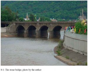
• Search for:
• Make a Gift
• Maps / Directions

Advertisement

Supported by

Dubai’s Extraordinary Flooding: Here’s What to Know

Images of a saturated desert metropolis startled the world, prompting talk of cloud seeding, climate change and designing cities for intensified weather.

• Share full article

By Raymond Zhong

Scenes of flood-ravaged neighborhoods in one of the planet’s driest regions have stunned the world this week. Heavy rains in the United Arab Emirates and Oman submerged cars, clogged highways and killed at least 21 people. Flights out of Dubai’s airport, a major global hub, were severely disrupted.

The downpours weren’t a freak event — forecasters anticipated the storms several days out and issued warnings. But they were certainly unusual. Here’s what to know.

Heavy rain there is rare, but not unheard-of.

On average, the Arabian Peninsula receives a scant few inches of rain a year, although scientists have found that a sizable chunk of that precipitation falls in infrequent but severe bursts, not as periodic showers.

U.A.E. officials said the 24-hour rain total on Tuesday was the country’s largest since records there began in 1949 . But parts of the nation had experienced an earlier round of thunderstorms just last month.

Oman, with its coastline on the Arabian Sea, is also vulnerable to tropical cyclones. Past storms there have brought torrential rain, powerful winds and mudslides, causing extensive damage.

Global warming is projected to intensify downpours.

Stronger storms are a key consequence of human-caused global warming. As the atmosphere gets hotter, it can hold more moisture, which can eventually make its way down to the earth as rain or snow.

But that doesn’t mean rainfall patterns are changing in precisely the same way across every corner of the globe.

In their latest assessment of climate research , scientists convened by the United Nations found there wasn’t enough data to have firm conclusions about rainfall trends in the Arabian Peninsula and how climate change was affecting them. The researchers said, however, that if global warming were to be allowed to continue worsening in the coming decades, extreme downpours in the region would quite likely become more intense and more frequent.

The role of cloud seeding isn’t clear.

The U.A.E. has for decades worked to increase rainfall and boost water supplies by seeding clouds. Essentially, this involves shooting particles into clouds to encourage the moisture to gather into larger, heavier droplets, ones that are more likely to fall as rain or snow.

Cloud seeding and other rain-enhancement methods have been tried across the world, including in Australia, China, India, Israel, South Africa and the United States. Studies have found that these operations can, at best, affect precipitation modestly — enough to turn a downpour into a bigger downpour, but probably not a drizzle into a deluge.

Still, experts said pinning down how much seeding might have contributed to this week’s storms would require detailed study.

“In general, it is quite a challenge to assess the impact of seeding,” said Luca Delle Monache, a climate scientist at the Scripps Institution of Oceanography in La Jolla, Calif. Dr. Delle Monache has been leading efforts to use artificial intelligence to improve the U.A.E.’s rain-enhancement program.

An official with the U.A.E.’s National Center of Meteorology, Omar Al Yazeedi, told news outlets this week that the agency didn’t conduct any seeding during the latest storms. His statements didn’t make clear, however, whether that was also true in the hours or days before.

Mr. Al Yazeedi didn’t respond to emailed questions from The New York Times on Thursday, and Adel Kamal, a spokesman for the center, didn’t immediately have further comment.

Cities in dry places just aren’t designed for floods.

Wherever it happens, flooding isn’t just a matter of how much rain comes down. It’s also about what happens to all that water once it’s on the ground — most critically, in the places people live.

Cities in arid regions often aren’t designed to drain very effectively. In these areas, paved surfaces block rain from seeping into the earth below, forcing it into drainage systems that can easily become overwhelmed.

One recent study of Sharjah , the capital of the third-largest emirate in the U.A.E., found that the city’s rapid growth over the past half century had made it vulnerable to flooding at far lower levels of rain than before.

Omnia Al Desoukie contributed reporting.

Raymond Zhong reports on climate and environmental issues for The Times. More about Raymond Zhong

What caused Dubai floods? Experts cite climate change, not cloud seeding

• Medium Text

DID CLOUD SEEDING CAUSE THE STORM?

CAN'T CREATE CLOUDS FROM NOTHING

Coming soon: Get the latest news and expert analysis about the state of the global economy with Reuters Econ World. Sign up here.

Reporting by Alexander Cornwell; editing by Maha El Dahan and Alexandra Hudson

Our Standards: The Thomson Reuters Trust Principles. New Tab , opens new tab

World Chevron

Iraq's Popular Mobilization Forces, an official security force, said its command post at Kalso military base about 50 km (30 miles) south of Baghdad was hit by a huge explosion late on Friday, and two security sources said it resulted from an air strike.

The United States will withdraw its troops from Niger, a source familiar with the matter told Reuters late on Friday, adding an agreement was reached between U.S Deputy Secretary of State Kurt Campbell and Niger's leadership.

Semyon Eremin, a war correspondent for the Russian daily Izvestia, was killed on Friday in a drone attack in southeastern Ukraine, the daily said.

Video Case Studies: PayPal Braintree offers cutting-edge functionality with proven reliability

PayPal Editorial Staff

April 18, 2024

As a subscription-based business, ensuring the continuity of the customer experience across all its brands is critical. Maintaining a customer’s desire to improve their health is key to their purchasing decision, so ease of checkout is paramount.

All in a single integration, PayPal Braintree enables Wellful to offer PayPal, Venmo, credit cards, and other alternative payment methods. Additional functions like network tokenization and real-time account updater help ensure secure transacting and up-to-date customer data.

We sat down with Wellful’s CTO Nitin Chaudhary and CEO Brandon Adcock to talk how the company sought a payment processor that could provide advanced technology and align with Wellful’s forward-looking approach. And with the ability to implement several payment methods quickly via a single integration.

Watch the testimonial videos to learn more about how a seamless checkout process removes any barriers that may dissuade their customers.

Learn more about How PayPal Braintree helped Wellful, Inc. increase approval rates .

Wellful Case Study (PDF)

Was this content helpful?

Related content

Sign up to stay informed.

Share your email to receive the latest enterprise updates, top stories, and industry reports.

*Required fields

I consent to PayPal contacting me by phone or by email, and to sending me product or industry information relevant to my query. I know I can unsubscribe at any time.

We use cookies to improve your experience on our site. May we use marketing cookies to show you personalized ads? Manage all cookies